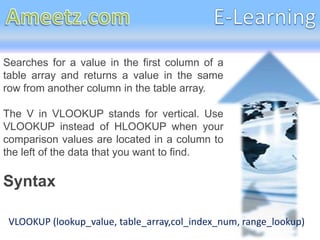
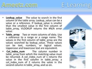
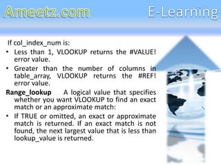
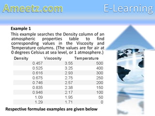
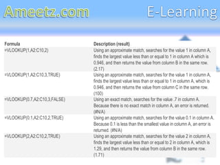
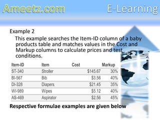
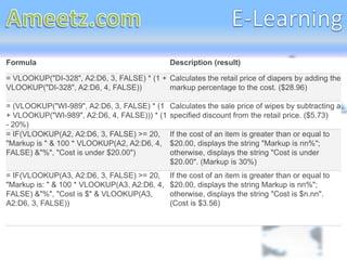
The document provides an overview of the VLOOKUP function in Excel, including its syntax and parameters such as lookup_value, table_array, col_index_num, and range_lookup. It explains how to use VLOOKUP to find data from a specific column based on a search value and provides examples for both approximate and exact matches. Additionally, it includes practical examples on calculating retail prices and displaying conditional strings based on item costs and markups.

1. Excel Tips and Tricks

2. Excel – Vlookup

3. Searches for a value in the first column of a
table array and returns a value in the same
row from another column in the table array.
The V in VLOOKUP stands for vertical. Use
VLOOKUP instead of HLOOKUP when your
comparison values are located in a column to
the left of the data that you want to find.
Syntax
VLOOKUP (lookup_value, table_array,col_index_num, range_lookup)

4. • Lookup_value The value to search in the first
column of the table array. Lookup_value can be a
value or a reference. If lookup_value is smaller
than the smallest value in the first column of
table_array, VLOOKUP returns the #N/A error
value.
• Table_array Two or more columns of data. Use
a reference to a range or a range name. The
values in the first column of table_array are the
values searched by lookup_value. These values
can be text, numbers, or logical values.
Uppercase and lowercase text are equivalent.
• Col_index_num The column number in
table_array from which the matching value must
be returned. A col_index_num of 1 returns the
value in the first column in table_array; a
col_index_num of 2 returns the value in the
second column in table_array, and so on.

5. If col_index_num is:
• Less than 1, VLOOKUP returns the #VALUE!
error value.
• Greater than the number of columns in
table_array, VLOOKUP returns the #REF!
error value.
Range_lookup A logical value that specifies
whether you want VLOOKUP to find an exact
match or an approximate match:
• If TRUE or omitted, an exact or approximate
match is returned. If an exact match is not
found, the next largest value that is less than
lookup_value is returned.

6. Example 1
This example searches the Density column of an
atmospheric properties table to find
corresponding values in the Viscosity and
Temperature columns. (The values are for air at
0 degrees Celsius at sea level, or 1 atmosphere.)
Respective formulae examples are given below

7. Formula Description (result)
=VLOOKUP(1,A2:C10,2) Using an approximate match, searches for the value 1 in column A,
finds the largest value less than or equal to 1 in column A which is
0.946, and then returns the value from column B in the same row.
(2.17)
=VLOOKUP(1,A2:C10,3,TRUE) Using an approximate match, searches for the value 1 in column A,
finds the largest value less than or equal to 1 in column A, which is
0.946, and then returns the value from column C in the same row.
(100)
=VLOOKUP(0.7,A2:C10,3,FALSE) Using an exact match, searches for the value .7 in column A.
Because there is no exact match in column A, an error is returned.
(#N/A)
=VLOOKUP(0.1,A2:C10,2,TRUE) Using an approximate match, searches for the value 0.1 in column A.
Because 0.1 is less than the smallest value in column A, an error is
returned. (#N/A)
=VLOOKUP(2,A2:C10,2,TRUE) Using an approximate match, searches for the value 2 in column A,
finds the largest value less than or equal to 2 in column A, which is
1.29, and then returns the value from column B in the same row.
(1.71)

8. Example 2
This example searches the Item-ID column of a baby
products table and matches values in the Cost and
Markup columns to calculate prices and test
conditions.
Item-ID Item Cost Markup
ST-340 Stroller $145.67 30%
BI-567 Bib $3.56 40%
DI-328 Diapers $21.45 35%
WI-989 Wipes $5.12 40%
AS-469 Aspirator $2.56 45%
Respective formulae examples are given below

9. Formula Description (result)
= VLOOKUP("DI-328", A2:D6, 3, FALSE) * (1 + Calculates the retail price of diapers by adding the
VLOOKUP("DI-328", A2:D6, 4, FALSE)) markup percentage to the cost. ($28.96)
= (VLOOKUP("WI-989", A2:D6, 3, FALSE) * (1 Calculates the sale price of wipes by subtracting a
+ VLOOKUP("WI-989", A2:D6, 4, FALSE))) * (1 specified discount from the retail price. ($5.73)
- 20%)
= IF(VLOOKUP(A2, A2:D6, 3, FALSE) >= 20, If the cost of an item is greater than or equal to
"Markup is " & 100 * VLOOKUP(A2, A2:D6, 4, $20.00, displays the string "Markup is nn%";
FALSE) &"%", "Cost is under $20.00") otherwise, displays the string "Cost is under
$20.00". (Markup is 30%)
= IF(VLOOKUP(A3, A2:D6, 3, FALSE) >= 20, If the cost of an item is greater than or equal to
"Markup is: " & 100 * VLOOKUP(A3, A2:D6, 4, $20.00, displays the string Markup is nn%";
FALSE) &"%", "Cost is $" & VLOOKUP(A3, otherwise, displays the string "Cost is $n.nn".
A2:D6, 3, FALSE)) (Cost is $3.56)