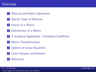
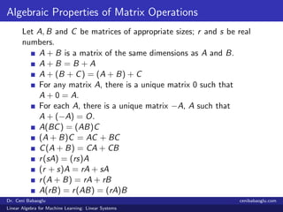
1. Linear Algebra for Machine Learning: Linear Systems

Seminar Series on
Linear Algebra for Machine Learning
Part 1: Linear Systems
Dr. Ceni Babaoglu
Ryerson University
cenibabaoglu.com
Dr. Ceni Babaoglu cenibabaoglu.com
Linear Algebra for Machine Learning: Linear Systems

Overview
1 Matrices and Matrix Operations
2 Special Types of Matrices
3 Inverse of a Matrix
4 Determinant of a Matrix
5 A statistical Application: Correlation Coeﬃcient
6 Matrix Transformations
7 Systems of Linear Equations
8 Linear Systems and Inverses
9 References

Matrices
An m × n matrix
A =





a11 a12 a13 . . . a1n
a21 a22 a23 . . . a2n
...
...
...
...
...
am1 am2 am3 . . . amn





= [aij ]
The i th row of A is
A = ai1 ai2 ai3 . . . ain , (1 ≤ i ≤ m)
The j th column of A is
A =





a1j
a2j
...
amj





, (1 ≤ j ≤ n)

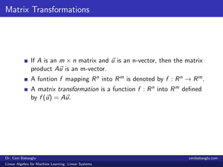
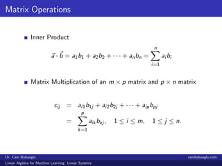
Matrix Operations
Matrix Addition
A + B = [aij ] + [bij ] , C = [cij ]
cij = aij + bij , i = 1, 2, · · · , m, j = 1, 2, · · · , n.
Scalar Multiplication
rA = r [aij ] , C = [cij ]
cij = r aij , i = 1, 2, · · · , m, j = 1, 2, · · · , n.
Transpose of a Matrix
AT
= aT
ij , aT
ij = aji

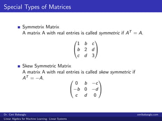
Special Types of Matrices
Diagonal Matrix
An n × n matrix A = [aij ] is called a diagonal matrix if aij = 0
for i = j 




a 0 . . . 0
0 1 . . . 0
...
...
...
...
0 0 . . . 1





Identity Matrix
The scalar matrix In = [dij ], where dii = 1 and dij = 0 for
i = j, is called the n × n identity matrix





1 0 . . . 0
0 1 . . . 0
...
...
...
...
0 0 . . . 1






Upper Triangular Matrix
An n × n matrix A = [aij ] is called upper triangular if aij = 0
for i > j 

2 b c
0 3 0
0 0 1


Lower Triangular Matrix
An n × n matrix A = [aij ] is called lower triangular if aij = 0
for i < j 

2 0 0
0 3 0
a b 1



Symmetrix Matrix
A matrix A with real entries is called symmetric if AT = A.


1 b c
b 2 d
c d 3


Skew Symmetric Matrix
A matrix A with real entries is called skew symmetric if
AT = −A. 

0 b −c
−b 0 −d
c d 0



Matrix Operations
Inner Product
a · b = a1b1 + a2b2 + · · · + anbn =
n
i=1
ai bi
Matrix Multiplication of an m × p matrix and p × n matrix
cij = ai1b1j + ai2b2j + · · · + aipbpj
=
p
k=1
aikbkj , 1 ≤ i ≤ m, 1 ≤ j ≤ n.

Algebraic Properties of Matrix Operations
Let A, B and C be matrices of appropriate sizes; r and s be real
numbers.
A + B is a matrix of the same dimensions as A and B.
A + B = B + A
A + (B + C) = (A + B) + C
For any matrix A, there is a unique matrix 0 such that
A + 0 = A.
For each A, there is a unique matrix −A, A such that
A + (−A) = O.
A(BC) = (AB)C
(A + B)C = AC + BC
C(A + B) = CA + CB
r(sA) = (rs)A
(r + s)A = rA + sA
r(A + B) = rA + rB
A(rB) = r(AB) = (rA)B

Inverse of a Matrix
Nonsingular Matrices
An n × n matrix is called nonsingular, or invertible if there
exists an n × n matrix B such that AB = BA = In.
Inverse Matrix
Such a B is called an inverse of A.
If such a B does not exist, A is called singular, or
noninvertible.
The inverse of a matrix, if it exists, is unique.
AA−1
= A−1
A = In
AA−1
=
1 2
3 4
−2 1
3/2 −1/2
=
−2 1
3/2 −1/2
1 2
3 4
=
1 0
0 1

Determinant of a Matrix
Associated with every square matrix A is a number called the
determinant, denoted by det(A). For 2 × 2 matrices, the
determinant is deﬁned as
A =
a b
c d
, det(A) = ad − bc
A =
2 1
−4 −2
, det(A) = (2)(−2) − (1)(−4) = 0

Properties of Determinants
1 If I is the identity, then det(I) = 1.
2 If B is obtained from A by interchanging two rows, then
det(B) = −det(A).
3 If B is obtained from A by adding a multiple of one row of A
to another row, then det(B) = det(A).
4 If B is obtained from A by multiplying a row of A by the
number m, then det(B) = m det(A).
5 Determinant of an upper (or lower) triangular matrix is equal
to the product of its diagonal entries.

Determinant of an n × n matrix
Minor
Suppose that in an n × n matrix A we delete the ith row and
jth column to obtain an (n − 1) × (n − 1) matrix. The
determinant of this sub-matrix is called the (i, j)th minor of A
and is denoted by Mij .
Cofactor
The number (−1)i+j Mij is called the (i, j)th cofactor of A
and is denoted by Cij .
Determinant
Let A be an n × n matrix. Then det(A) can be evaluated by
expanding by cofactors along any row or any column:
det(A) = ai1Ci1 + ai2Ci2 + · · · + ainCin, 1 ≤ i ≤ n.
or
det(A) = a1j C1j + a2j C2j + · · · + anj Cnj , 1 ≤ j ≤ n.

Example
Let’s ﬁnd the determinant of the following matrix.
A =


2 −3 1
4 0 −2
3 −1 −3

 .
If we expand cofactors along the ﬁrst row:
|A| = (2)C11 + (−3)C12 + (1)C13
= 2(−1)1+1 0 −2
−1 −3
− 3(−1)1+2 4 −2
3 −3
+ 1(−1)1+3 4 0
3 −1
= 2(−2) + 3(−6) + (−4) = −26.
If we expand along the third column, we obtain
|A| = (1)C13 + (−2)C23 + (−3)C33
= 1(−1)1+3 4 0
3 −1
− 2(−1)2+3 2 −3
3 −1
− 3(−1)3+3 2 −3
4 0
= −26.

Angle between to vectors
The length of n-vector
v =







v1
v2
...
vn−1
vn







is deﬁnes as
v = v2
1 + v2
2 + · · · + v2
n−1 + v2
n .
The angle between the two nonzero vectors is determined by
cos(θ) =
u · v
u v
.
−1
u · v
u v
1, 0 θ π

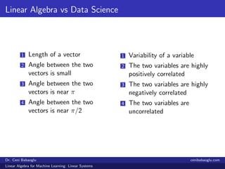
A statistical application: Correlation Coeﬃcient
Sample means of two attributes
¯x =
1
n
n
i=1
x, ¯y =
1
n
n
i=1
y
Centered form
xc = [x1 − ¯x x2 − ¯x · · · xn − ¯x]T
yc = [y1 − ¯y y2 − ¯y · · · yn − ¯y]T
Correlation coeﬃcient
Cor(xc, yc) =
xc · yc
xc yc
r =
n
i=1(xi − ¯x)(yi − ¯y)
n
i=1(xi − ¯x)2 n
i=1(yi − ¯y)2

Linear Algebra vs Data Science
1 Length of a vector
2 Angle between the two
vectors is small
vectors is near π
vectors is near π/2
1 Variability of a variable
2 The two variables are highly
positively correlated
3 The two variables are highly
negatively correlated
4 The two variables are
uncorrelated

Matrix Transformations
If A is an m × n matrix and u is an n-vector, then the matrix
product Au is an m-vector.
A funtion f mapping Rn into Rm is denoted by f : Rn → Rm.
A matrix transformation is a function f : Rn into Rm deﬁned
by f (u) = Au.

Example
Let f : R2 → R2 be the matrix transformation defined by
f (u) =
1 0
0 −1
u.
f (u) = f
x
y
=
1 0
0 −1
x
y
=
x
−y
This transformation performs a reflection with respect to the x-axis
in R2.
To see a reflection of a point, say (2,-3)
1 0
0 −1
2
−3
=
2
3

Systems of Linear Equations
A linear equation in variables x1, x2, . . . , xn is an equation of the
form
a1x1 + a2x2 + . . . + anxn = b.
A collection of such equations is called a linear system:
a11x1 + a12x2 + · · · + a1nxn = b1
a21x1 + a22x2 + · · · + a2nxn = b2
...
...
...
...
am1x1 + am2x2 + · · · + amnxn = bm

Systems of Linear Equations
For the system of equations
a11x1 + a12x2 + · · · + a1nxn = b1
a21x1 + a22x2 + · · · + a2nxn = b2
...
...
...
...
am1x1 + am2x2 + · · · + amnxn = bm
Ax = b
The augmented matrix:




a11 a12 a13 . . . a1n b1
a21 a22 a23 . . . a2n b2
. . . . . . . . . . . . . . . . . .
am1 am2 am3 . . . amn bm




If b1 = b2 = · · · = bm = 0, the system is called homogeneous.
Ax = 0

Linear Systems and Inverses
If A is an n × n matrix, then the linear system Ax = b is a system
of n equations in n unknowns.
Suppose that A is nonsingular.
Ax = b
A−1
(Ax) = A−1
b
(A−1
A)x = A−1
b
Inx = A−1
b
x = A−1
b
x = A−1b is the unique solution of the linear system.

Solving Linear Systems
A matrix is in echelon form if
1 All zero rows, if there are any, appear at the bottom of the
matrix.
2 The ﬁrst nonzero entry from the left of a nonzero row is a 1.
This entry is called a leading one of its row.
3 For each nonzero row, the leading one appears to the right
and below any leading ones in preceding rows.
4 If a column contains a leading one, then all other entries in
that column are zero.



1 0 0 0
0 1 0 0
0 0 1 0
0 0 0 1








1 0 0 0 1 3
0 1 0 0 5 2
0 0 0 1 2 0
0 0 0 0 0 0








1 2 0 0 3
0 0 1 0 2
0 0 0 0 0
0 0 0 0 0





An elementary row operation on a matrix is one of the following:
1 interchange two rows,
2 add a multiple of one row to another, and
3 multiply one row by a non-zero constant.
Two matrices are row equivalent if one can be converted into
the other through a series of elementary row operations.
Every matrix is row equivalent to a matrix in echelon form.

If an augmented matrix is in echelon form, then the ﬁrst
nonzero entry of each row is a pivot.
The variables corresponding to the pivots are called pivot
variables, and the other variables are called free variables.
A matrix is in reduced echelon form if all pivot entries are 1
and all entries above and below the pivots are 0.
A system of linear equations with more unknowns than
equations will either fail to have any solutions or will have an
inﬁnite number of solutions.

Example: Let’s solve the following system.
x1 − 3 x2 + x3 = 1
2 x1 + x2 − x3 = 2
4 x1 + 4 x2 − 2 x3 = 1
5 x1 − 8 x2 + 2 x3 = 5




1 −3 1
2 1 −1
4 4 −2
5 −8 2
1
2
1
5




R2−2R1→R2
R3−4R1→R3
R4−5R1→R4
−−−−−−−→




1 −3 1
0 7 −3
0 16 −6
0 7 −3
1
0
−3
0




R2/7→R2
−−−−−→




1 −3 1
0 1 −3/7
0 16 −6
0 7 −3
1
0
−3
0




R1+3R2→R1
R3−16R2→R3
R4−7R2→R4
−−−−−−−−→




1 0 −2/7
0 1 −3/7
0 0 6/7
0 0 0
1
0
−3
0




7R3/6→R3
−−−−−−→




1 0 −2/7
0 1 −3/7
0 0 1
0 0 0
1
0
−7/2
0




R1+2R3/7→R1
R2+3R3/7→R2
−−−−−−−−→




1 0 0
0 1 0
0 0 1
0 0 0
0
−3/2
−7/2
0




⇔ x1 = 0, x2 = −3/2, x3 = −7/2

Example: Let’s solve the following homogenous system.
2 x1 + 4 x2 + 3 x3 + 3 x4 + 3 x5 = 0
x1 + 2 x2 + x3 + 2 x4 + x5 = 0
x1 + 2 x2 + 2 x3 + x4 + 2 x5 = 0
x3 − x4 − x5 = 0




2 4 3 3 3
1 2 1 2 1
1 2 2 1 2
0 0 1 −1 −1
0
0
0
0




R1↔R2
−−−−→




1 2 1 2 1
2 4 3 3 3
1 2 2 1 2
0 0 1 −1 −1
0
0
0
0




R2−2R1→R2
R3−R1→R3
−−−−−−−→




1 2 1 2 1
0 0 1 −1 1
0 0 1 −1 1
0 0 1 −1 −1
0
0
0
0




R3−R2→R3
R4−R2→R4
−−−−−−−→




1 2 1 2 1
0 0 1 −1 1
0 0 0 0 0
0 0 0 0 −2
0
0
0
0




R3↔R4
−−−−→




1 2 1 2 1
0 0 1 −1 1
0 0 0 0 −2
0 0 0 0 0
0
0
0
0




−R3/2→R3
−−−−−−−→




1 2 1 2 1
0 0 1 −1 1
0 0 0 0 1
0 0 0 0 0
0
0
0
0




x1 + 2x2 + x3 + 2x4 + x5 = 0, x3 − x4 + x5 = 0
x5 = 0, x2 = α, x4 = β, x3 = β, x1 = −2α − β − 2β.

Example: Let’s use elementary row operations to ﬁnd A−1
if
A =


4 3 2
5 6 3
3 5 2

.


4 3 2
5 6 3
3 5 2
1 0 0
0 1 0
0 0 1

 R1−R3→R1
−−−−−−−→


1 −2 0
5 6 3
3 5 2
1 0 −1
0 1 0
0 0 1


R2−5R1→R2
R3−3R1→R3
−−−−−−−→


1 −2 0
0 16 3
0 11 2
1 0 −1
−5 1 5
−3 0 4

 R2/16→R2
−−−−−−→


1 −2 0
0 1 3/16
0 11 2
1 0 −1
−5/16 1/16 5/16
−3 0 4


R1+2R2→R1R3−11R1→R3
−−−−−−−−−−−−−−−→


1 0 3/8
0 1 3/16
0 0 −1/16
3/8 1/8 −3/8
−5/16 1/16 5/16
7/16 −11/16 9/16


R1+6R3→R1
R2+3R3→R2
−−−−−−−→


1 0 0
0 1 0
0 0 −1/16
3 −4 3
1 −2 2
7/16 −11/16 9/16

 −16R3→R3
−−−−−−→


1 0 0
0 1 0
0 0 1
3 −4 3
1 −2 2
−7 11 −9


A−1
=


3 −4 3
1 −2 2
−7 11 −9



References
Linear Algebra With Applications, 7th Edition
by Steven J. Leon.
Elementary Linear Algebra with Applications, 9th Edition
by Bernard Kolman and David Hill.

1. Linear Algebra for Machine Learning: Linear Systems

More Related Content

What's hot

Similar to 1. Linear Algebra for Machine Learning: Linear Systems

Recently uploaded

1. Linear Algebra for Machine Learning: Linear Systems