1. Introduction to MATLAB 2. Linear algebra refresher 3. Writing fast MATLAB code

1. Linear Algebra and MATLAB Tutorial
Jia-Bin Huang
University of Illinois, Urbana-Champaign
www.jiabinhuang.com
jbhuang1@Illinois.edu

2. Today’s class
• Introduction to MATLAB
• Linear algebra refresher
• Writing fast MATLAB code

3. Working with MATLAB

4. Learning by doing
• Let’s work through an example!
• Download the example script here
• Topics
• Basic types in Matlab
• Operations on vectors and matrices
• Control statements & vectorization
• Saving/loading your work
• Creating scripts or functions using m-files
• Plotting
• Working with images

5. Questions?

6. Linear algebra refresher
• Linear algebra is the math tool du jour
• Compact notation
• Convenient set operations
• Used in all modern texts
• Interfaces well with MATLAB, numpy, R, etc.
• We will use a lot of it!!
Slides credits: Paris Smaragdis and Karianne Bergen

7. Filtering, linear transformation
-> extracting frequency sub-bands
Vector dot products
-> measure patch similarities
Hybrid Image Image Quilting Gradient Domain Fusion
Solving linear systems
-> solve for pixel values
Image-based Lighting
Solving linear systems -> solve for radiance map
Video Stitching and Processing
Solving linear systems -> solve for geometric transform

8. Scalars, Vectors, Matrices, Tensors

9. How will we see these?
• Vector: an ordered collection of scalars (e.g., sounds)
• Matrix: a two-dimensional collection of scalars (e.g., images)
• Tensor: 3D signals (e.g., videos)

10. Element-wise operations
• Addition/subtraction
• 𝒂 ± 𝒃 = 𝒄 ⇒ 𝑎𝑖 + 𝑏𝑖 = 𝑐𝑖
• Multiplication (Hadamard product)
• 𝒂 𝒃 = 𝒄 ⇒ 𝑎𝑖 𝑏𝑖 = 𝑐𝑖
• No named operator for element-wise division
• Just use Hadamard with inverted elements
c = a + b;
c = a – b;
c = a.*b;
c = a./b;

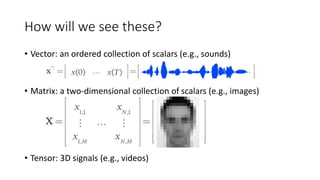
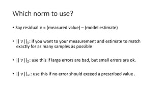
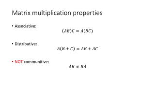
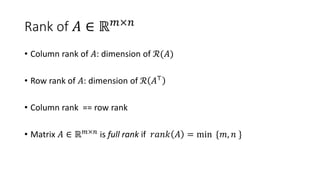
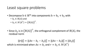
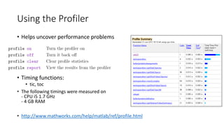
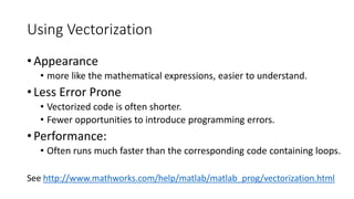
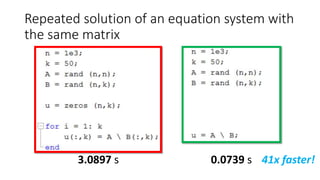
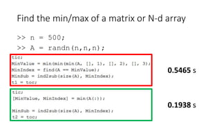
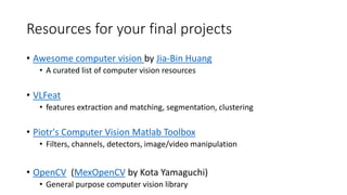
11. Which division?
Left Right
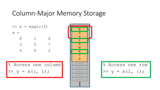
Array division C = ldivide(A, B);
C = A.B;
C = rdivide(A, B);
C = A./B;
Matrix division C = mldivide(A, B);
C = A/B;
C = mldivide(A, B);
C = AB;
EX: Array division
A = [1 2; 3, 4];
B = [1,1; 1, 1];
C1 = A.B;
C2 = A./B;
C1 =
1.0000 0.5000
0.3333 0.2500
C2 =
1 2
3 4
EX: Matrix division
X = AB;
-> the (least-square) solution to AX = B
X = A/B;
-> the (least-square) solution to XB = A
B/A = (A'B')'

12. Transpose
• Change rows to columns (and vice versa)
• Hermitian (conjugate transpose)
• Notated as 𝑋H
• Y = X’; % Hermitian transpose
• Y = X.’; % Transpose (without conjugation)

13. Visualizing transposition
• Mostly pointless for 1D signals
• Swap dimensions for 2D signals

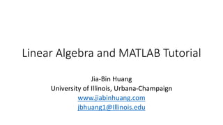
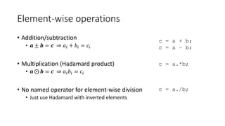
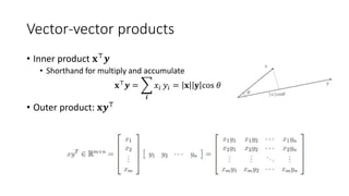
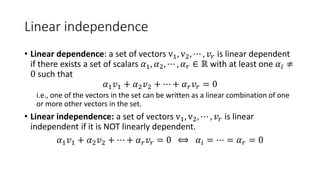
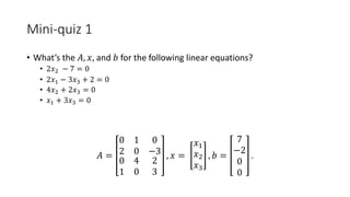
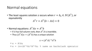
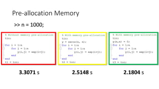
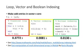
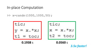
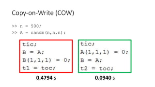
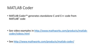
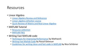
14. Reshaping operators
• The vec operator
• Unrolls elements column-wise
• Useful for getting rid of matrices/tensors
• B = A(:);
• The reshape operator
• B = reshape(A, sz);
• prod(sz) must be the same as
numel(A)
EX: Reshape
A = 1:12;
B = reshape(A,[3,4]);
B =
1 4 7 10
2 5 8 11
3 6 9 12

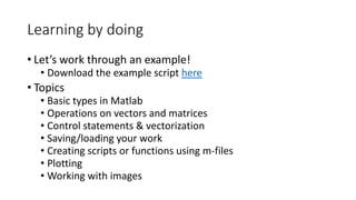
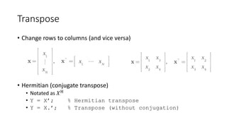
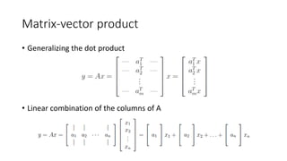
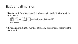
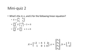
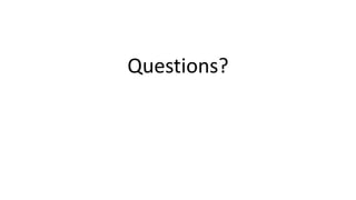
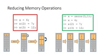
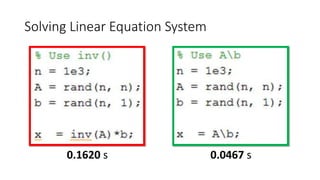
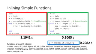
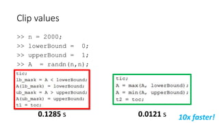
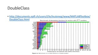
15. Trace and diag
• Matrix trace
• Sum of diagonal elements
• The diag operator EX: trace
A = [1, 2; 3, 4];
t = trace(A);
Q: What’s t?
EX: diag
x = diag(A);
D = diag(x);
Q: What’s x and D?

16. Vector norm (how “big" a vector is)
• Taxicab norm or Manhattan norm
• | 𝑣 | 1 = ∑|𝑣𝑖|
• Euclidean norm
• | 𝑣 | 2 = ∑𝑣𝑖
2
1
2 = 𝑣⊤ 𝑣
• Infinity norm
• | 𝑣 | ∞ = max
𝑖
|𝑣𝑖|
• P-norm
• | 𝑣 | 𝑝 = ∑𝑣𝑖
𝑝
1
𝑝
Unit circle
(the set of all vectors of norm 1)

17. Which norm to use?
• Say residual 𝑣 = (measured value) – (model estimate)
• | 𝑣 | 1: if you want to your measurement and estimate to match
exactly for as many samples as possible
• | 𝑣 | 2: use this if large errors are bad, but small errors are ok.
• | 𝑣 | ∞: use this if no error should exceed a prescribed value .

18. Vector-vector products
• Inner product 𝐱⊤ 𝒚
• Shorthand for multiply and accumulate
𝐱⊤ 𝒚 =
𝒊
𝑥𝑖 𝑦𝑖 = 𝐱 𝐲 cos 𝜃
• Outer product: 𝐱𝒚⊤

19. Matrix-vector product
• Generalizing the dot product
• Linear combination of the columns of A

20. Matrix-matrix product C = AB
Definition: as inner products
𝐶𝑖𝑗 = 𝑎𝑖
⊤
𝑏𝑗
As sum of outer productsAs a set of matrix-vector products
• matrix 𝐴 and columns of B
• rows of 𝐴 and matrix B

21. Matrix products
• Output rows == left matrix rows
• Output columns == right matrix columns

22. Matrix multiplication properties
• Associative:
𝐴𝐵 𝐶 = 𝐴(𝐵𝐶)
• Distributive:
𝐴 𝐵 + 𝐶 = 𝐴𝐵 + 𝐴𝐶
• NOT communitive:
𝐴𝐵 ≠ 𝐵𝐴

23. Linear independence
• Linear dependence: a set of vectors v1, v2, ⋯ , 𝑣𝑟 is linear dependent
if there exists a set of scalars 𝛼1, 𝛼2, ⋯ , 𝛼 𝑟 ∈ ℝ with at least one 𝛼𝑖 ≠
0 such that
𝛼1 𝑣1 + 𝛼2 𝑣2 + ⋯ + 𝛼 𝑟 𝑣𝑟 = 0
i.e., one of the vectors in the set can be written as a linear combination of one
or more other vectors in the set.
• Linear independence: a set of vectors v1, v2, ⋯ , 𝑣𝑟 is linear
independent if it is NOT linearly dependent.
𝛼1 𝑣1 + 𝛼2 𝑣2 + ⋯ + 𝛼 𝑟 𝑣𝑟 = 0 ⟺ 𝛼𝑖 = ⋯ = 𝛼 𝑟 = 0

24. Basis and dimension
• Basis: a basis for a subspace 𝑆 is a linear independent set of vectors
that span 𝑆
•
1
0
,
0
1
and
1
−1
,
1
1
are both bases that span ℝ2
• Not unique
• Dimension dim(𝑆): the number of linearly independent vectors in the
basis for 𝑆

25. Range and nullspace of a matrix 𝐴 ∈ ℝ 𝑚×𝑛
• The range (column space, image) of a matrix 𝐴 ∈ ℝ 𝑚×𝑛
• Denoted by ℛ(𝐴)
• The set of all linear combination of the columns of 𝐴
ℛ 𝐴 = 𝐴𝑥 𝑥 ∈ ℝ 𝑛
}, ℛ(𝐴) ⊆ ℝ 𝑚
• The nullspace (kernel) of a matrix 𝐴 ∈ ℝ 𝑚×𝑛
• Denoted by 𝒩(𝐴)
• The set of vectors z such that 𝐴𝑧 = 0
𝒩 𝐴 = { 𝑧 ∈ ℝ 𝑛|𝐴𝑧 = 0}, 𝒩 𝐴 ⊆ ℝ 𝑚

26. Rank of 𝐴 ∈ ℝ 𝑚×𝑛
• Column rank of 𝐴: dimension of ℛ(𝐴)
• Row rank of 𝐴: dimension of ℛ 𝐴⊤
• Column rank == row rank
• Matrix 𝐴 ∈ ℝ 𝑚×𝑛 is full rank if 𝑟𝑎𝑛𝑘 𝐴 = min {𝑚, 𝑛 }

27. System of linear equations
• Ex: Find values 𝑥1, 𝑥2, 𝑥3 ∈ ℝ that satisfy
• 3𝑥1 + 2𝑥2 − 𝑥3 − 1 = 0
• 2𝑥1 − 2𝑥2 + 𝑥3 + 2 = 0
• −𝑥1 −
1
2
𝑥2 − 𝑥3 = 0
Solution:
• Step 1: write the system of linear equations as a matrix equation
𝐴 =
3 2 −1
2 −2 1
−1 −
1
2
−1
, 𝑥 =
𝑥1
𝑥2
𝑥3
, 𝑏 =
1
−2
0
.
• Step 2: Solve for 𝐴𝑥 = 𝑏

28. Mini-quiz 1
• What’s the 𝐴, 𝑥, and 𝑏 for the following linear equations?
• 2𝑥2 − 7 = 0
• 2𝑥1 − 3𝑥3 + 2 = 0
• 4𝑥2 + 2𝑥3 = 0
• 𝑥1 + 3𝑥3 = 0
𝐴 =
0 1 0
2 0 −3
0
1
4
0
2
3
, 𝑥 =
𝑥1
𝑥2
𝑥3
, 𝑏 =
7
−2
0
0
.

29. Mini-quiz 2
• What’s the 𝐴, 𝑥, and 𝑏 for the following linear equation?
• 𝑋 =
𝑥1 𝑥3
𝑥2 𝑥4
•
1
2
⊤
𝑋
−2
1
− 3 = 0
•
1
0
⊤
𝑋
1
1
+ 1 = 0
𝐴 =
−2 − 4 1 2
1 0 1 0
, 𝑥 =
𝑥1
𝑥2
𝑥3
𝑥4
, 𝑏 =
3
−1

30. Solving system of linear equations
• Given 𝐴 ∈ ℝ 𝑚×𝑛 and b ∈ ℝ 𝑚, find x ∈ ℝ 𝑛 such that 𝐴𝑥 = 𝑏
• Special case: a square matrix 𝐴 ∈ ℝ 𝑛×𝑛
• The solution: 𝐴−1 𝑏
• The matrix inverse A−1exists and is unique if and only if
• 𝐴 is a squared matrix of full rank
• “Undoes” a matrix multiplication
• 𝐴−1 𝐴 = 𝐼
• 𝐴−1 𝐴𝑌 = 𝑌
• Y𝐴𝐴−1 = 𝑌

31. Least square problems
• What if 𝑏 ∉ ℛ(𝐴)?
• No solution 𝑥 exists such that 𝐴𝑥 = 𝑏
• Least Squares problem:
• Define residual 𝑟 = 𝐴𝑥 − 𝑏
• Find vector 𝑥 ∈ ℝ 𝑛 that minimizes
||𝑟||2
2
=||𝐴𝑥 − 𝑏||2
2

32. Least square problems
• Decompose b ∈ ℝm into components b = b1 + b2 with
• 𝑏1 ∈ ℛ(𝐴) and
• 𝑏2 ∈ 𝒩 A⊤ = ℛ A
⊥
.
• Since 𝑏2 is in ℛ A
⊥
, the orthogonal complement of ℛ A , the
residual norm
||𝑟||2
2
= ||𝐴𝑥 − 𝑏1 − 𝑏2||2
2
= ||𝐴𝑥 − 𝑏1||2
2
+ ||𝑏2||2
2
which is minimized when 𝐴𝑥 = 𝑏1 and 𝑟 = 𝑏2 ∈ 𝒩 A⊤

33. Normal equations
• The least squares solution 𝑥 occurs when 𝑟 = 𝑏2 ∈ 𝒩 A⊤ , or
equivalently
𝐴⊤ 𝑟 = 𝐴⊤ 𝑏 − 𝐴𝑥 = 0
• Normal equations: 𝐴⊤ 𝐴𝑥 = 𝐴⊤ 𝑏
• If 𝐴 has full column rank, then 𝐴⊤ 𝐴 is invertible.
• Thus (𝐴⊤ 𝐴)𝑥 = (𝐴⊤ 𝑏) has a unique solution
𝑥 = (𝐴⊤ 𝐴)−1 𝐴⊤ 𝑏
• x = Ab;
• x = inv(A’*A)*A’*b; % same as backslash operator

34. Questions?

35. Writing Fast MATLAB Code

36. Using the Profiler
• Helps uncover performance problems
• Timing functions:
• tic, toc
• The following timings were measured on
- CPU i5 1.7 GHz
- 4 GB RAM
• http://www.mathworks.com/help/matlab/ref/profile.html

37. Pre-allocation Memory
3.3071 s
>> n = 1000;
2.1804 s2.5148 s

38. Reducing Memory Operations
>> x = 4;
>> x(2) = 7;
>> x(3) = 12;
>> x = zeros(3,1);
>> x = 4;
>> x(2) = 7;
>> x(3) = 12;

39. Vectorization
2.1804 s 0.0157 s
139x faster!

40. Using Vectorization
• Appearance
• more like the mathematical expressions, easier to understand.
• Less Error Prone
• Vectorized code is often shorter.
• Fewer opportunities to introduce programming errors.
• Performance:
• Often runs much faster than the corresponding code containing loops.
See http://www.mathworks.com/help/matlab/matlab_prog/vectorization.html

41. Binary Singleton Expansion Function
• Make each column in A zero mean
>> n1 = 5000;
>> n2 = 10000;
>> A = randn(n1, n2);
• See http://blogs.mathworks.com/loren/2008/08/04/comparing-repmat-and-bsxfun-
performance/
0.2994 s 0.2251 s
Why bsxfun is faster than repmat?
- bsxfun handles replication of the array
implicitly, thus avoid memory allocation
- Bsxfun supports multi-thread

42. Loop, Vector and Boolean Indexing
• Make odd entries in vector v zero
• n = 1e6;
• See http://www.mathworks.com/help/matlab/learn_matlab/array-indexing.html
• See Fast manipulation of multi-dimensional arrays in Matlab by Kevin Murphy
0.3772 s 0.0081 s 0.0130 s

43. Solving Linear Equation System
0.1620 s 0.0467 s

44. Dense and Sparse Matrices
• Dense: 16.1332 s
• Sparse: 0.0040 s
More than 4000x faster!
Useful functions:
sparse(),
spdiags(),
speye(), kron().0.6424 s 0.1157 s

45. Repeated solution of an equation system with
the same matrix
3.0897 s 0.0739 s 41x faster!

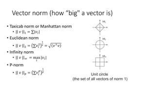
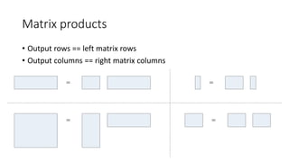
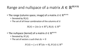
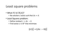
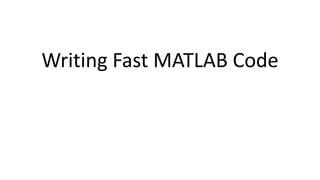
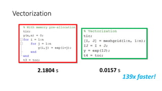
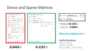
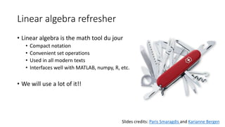
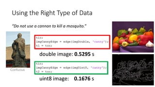
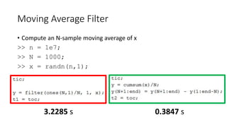
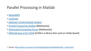
46. Iterative Methods for Larger Problems
• Iterative solvers in MATLAB:
• bicg, bicgstab, cgs, gmres, lsqr, minres, pcg, symmlq, qmr
• [x,flag,relres,iter,resvec] = method(A,b,tol,maxit,M1,M2,x0)
• source: Writing Fast Matlab Code by Pascal Getreuer

47. Solving Ax = b when A is a Special Matrix
• Circulant matrices
• Matrices corresponding to cyclic convolution
Ax = conv(h, x) are diagonalized in the Fourier domain
>> x = ifft( fft(b)./fft(h) );
• Triangular and banded
• Efficiently solved by sparse LU factorization
>> [L,U] = lu(sparse(A));
>> x = U(Lb);
• Poisson problems
• See http://www.cs.berkeley.edu/~demmel/cs267/lecture25/lecture25.html

48. In-place Computation
>> x=randn(1000,1000,50);
0.1938 s 0.0560 s
3.5x faster!

49. Inlining Simple Functions
1.1942 s 0.3065 s
functions are worth inlining:
- conv, cross, fft2, fliplr, flipud, ifft, ifft2, ifftn, ind2sub, ismember, linspace, logspace, mean,
median, meshgrid, poly, polyval, repmat, roots, rot90, setdiff, setxor, sortrows, std, sub2ind,
union, unique, var
y = medfilt1(x,5); 0.2082 s

50. Using the Right Type of Data
“Do not use a cannon to kill a mosquito.”
double image: 0.5295 s
uint8 image: 0.1676 s
Confucius

51. Matlab Organize its Arrays as Column-Major
• Assign A to zero row-by-row or column-by-column
>> n = 1e4;
>> A = randn(n, n);
0.1041 s2.1740 s 21x faster!

52. Column-Major Memory Storage
>> x = magic(3)
x =
8 1 6
3 5 7
4 9 2
% Access one column
>> y = x(:, 1);
% Access one row
>> y = x(1, :);

53. Copy-on-Write (COW)
>> n = 500;
>> A = randn(n,n,n);
0.4794 s 0.0940 s

54. Clip values
>> n = 2000;
>> lowerBound = 0;
>> upperBound = 1;
>> A = randn(n,n);
0.0121 s0.1285 s 10x faster!

55. Moving Average Filter
• Compute an N-sample moving average of x
>> n = 1e7;
>> N = 1000;
>> x = randn(n,1);
3.2285 s 0.3847 s

56. Find the min/max of a matrix or N-d array
>> n = 500;
>> A = randn(n,n,n);
0.5465 s
0.1938 s

57. Acceleration using MEX (Matlab Executable)
• Call your C, C++, or Fortran codes from the MATLAB
• Speed up specific subroutines
• See http://www.mathworks.com/help/matlab/matlab_external/introducing-mex-
files.html

58. MATLAB Coder
• MATLAB Coder™ generates standalone C and C++ code from
MATLAB® code
• See video examples in http://www.mathworks.com/products/matlab-
coder/videos.html
• See http://www.mathworks.com/products/matlab-coder/

59. DoubleClass
• http://documents.epfl.ch/users/l/le/leuteneg/www/MATLABToolbox/
DoubleClass.html

60. parfor for parallel processing
• Requirements
• Task independent
• Order independent
See http://www.mathworks.com/products/parallel-computing/

61. Parallel Processing in Matlab
• MatlabMPI
• multicore
• pMatlab: Parallel Matlab Toolbox
• Parallel Computing Toolbox (Mathworks)
• Distributed Computing Server (Mathworks)
• MATLAB plug-in for CUDA (CUDA is a library that used an nVidia board)
• Source: http://www-h.eng.cam.ac.uk/help/tpl/programs/Matlab/faster_scripts.html

62. Resources for your final projects
• Awesome computer vision by Jia-Bin Huang
• A curated list of computer vision resources
• VLFeat
• features extraction and matching, segmentation, clustering
• Piotr's Computer Vision Matlab Toolbox
• Filters, channels, detectors, image/video manipulation
• OpenCV (MexOpenCV by Kota Yamaguchi)
• General purpose computer vision library

63. Resources
• Linear Algebra
• Linear Algebra Review and Reference
• Linear algebra refresher course
• Quick Review of Matrix and Real Linear Algebra
• MATLAB Tutorial
• Resource collection
• MATLAB F&Q
• Writing Fast MATLAB code
• Techniques for Improving Performance by Mathwork
• Writing Fast Matlab Code by Pascal Getreuer
• Guidelines for writing clean and fast code in MATLAB by Nico Schlömer