This document contains lecture notes on linear algebra. It covers topics such as matrices, systems of linear equations, vector spaces, linear transformations, inner product spaces, eigenvalues and eigenvectors. The notes are divided into multiple chapters, with each chapter covering key concepts, definitions, theorems and examples for the topic. Methods for solving systems of linear equations like Gaussian elimination and Gauss-Jordan elimination are presented. Concepts such as subspaces, linear independence, bases and dimensions of vector spaces are defined. Linear transformations, change of basis, orthogonality and diagonalization are also discussed in detail.


![Chapter 1
Introduction to Matrices
1.1 Definition of a Matrix
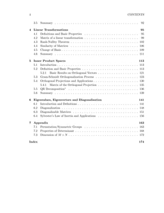
Definition 1.1.1 (Matrix). A rectangular array of numbers is called a matrix.
The horizontal arrays of a matrix are called its rows and the vertical arrays are called
its columns. A matrix is said to have the order m × n if it has m rows and n columns.
An m × n matrix A can be represented in either of the following forms:
A =
a11 a12 · · · a1n
a21 a22 · · · a2n
...
...
...
...
am1 am2 · · · amn
or A =
a11 a12 · · · a1n
a21 a22 · · · a2n
...
...
...
...
am1 am2 · · · amn
,
where aij is the entry at the intersection of the ith row and jth column. In a more concise
manner, we also write Am×n = [aij] or A = [aij]m×n or A = [aij]. We shall mostly
be concerned with matrices having real numbers, denoted R, as entries. For example, if
A =
1 3 7
4 5 6
then a11 = 1, a12 = 3, a13 = 7, a21 = 4, a22 = 5, and a23 = 6.
A matrix having only one column is called a column vector; and a matrix with
only one row is called a row vector. Whenever a vector is used, it should
be understood from the context whether it is a row vector or a column
vector. Also, all the vectors will be represented by bold letters.
Definition 1.1.2 (Equality of two Matrices). Two matrices A = [aij] and B = [bij] having
the same order m × n are equal if aij = bij for each i = 1, 2, . . . , m and j = 1, 2, . . . , n.
In other words, two matrices are said to be equal if they have the same order and their
corresponding entries are equal.
Example 1.1.3. The linear system of equations 2x + 3y = 5 and 3x + 2y = 5 can be
identified with the matrix
2 3 : 5
3 2 : 5
. Note that x and y are indeterminate and we can
think of x being associated with the first column and y being associated with the second
column.
5](https://image.slidesharecdn.com/booklinear-160914134339/85/Book-linear-5-320.jpg)
![6 CHAPTER 1. INTRODUCTION TO MATRICES
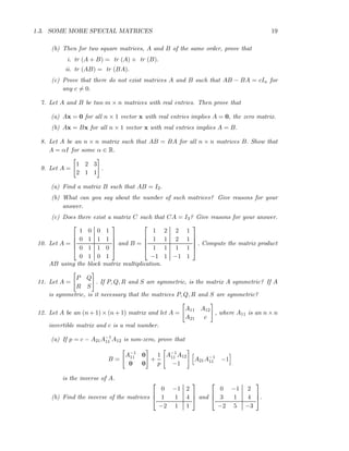
1.1.1 Special Matrices
Definition 1.1.4. 1. A matrix in which each entry is zero is called a zero-matrix, de-
noted by 0. For example,
02×2 =
0 0
0 0
and 02×3 =
0 0 0
0 0 0
.
2. A matrix that has the same number of rows as the number of columns, is called a
square matrix. A square matrix is said to have order n if it is an n × n matrix.
3. The entries a11, a22, . . . , ann of an n×n square matrix A = [aij] are called the diagonal
entries (the principal diagonal) of A.
4. A square matrix A = [aij] is said to be a diagonal matrix if aij = 0 for i = j. In
other words, the non-zero entries appear only on the principal diagonal. For example,
the zero matrix 0n and
4 0
0 1
are a few diagonal matrices.
A diagonal matrix D of order n with the diagonal entries d1, d2, . . . , dn is denoted by
D = diag(d1, . . . , dn). If di = d for all i = 1, 2, . . . , n then the diagonal matrix D is
called a scalar matrix.
5. A scalar matrix A of order n is called an identity matrix if d = 1. This matrix is
denoted by In.
For example, I2 =
1 0
0 1
and I3 =
1 0 0
0 1 0
0 0 1
. The subscript n is suppressed in
case the order is clear from the context or if no confusion arises.
6. A square matrix A = [aij] is said to be an upper triangular matrix if aij = 0 for
i > j.
A square matrix A = [aij] is said to be a lower triangular matrix if aij = 0 for
i < j.
A square matrix A is said to be triangular if it is an upper or a lower triangular
matrix.
For example,
0 1 4
0 3 −1
0 0 −2
is upper triangular,
0 0 0
1 0 0
0 1 1
is lower triangular.
Exercise 1.1.5. Are the following matrices upper triangular, lower triangular or both?
1.
a11 a12 · · · a1n
0 a22 · · · a2n
...
...
...
...
0 0 · · · ann
](https://image.slidesharecdn.com/booklinear-160914134339/85/Book-linear-6-320.jpg)
![1.2. OPERATIONS ON MATRICES 7
2. The square matrices 0 and I or order n.
3. The matrix diag(1, −1, 0, 1).
1.2 Operations on Matrices
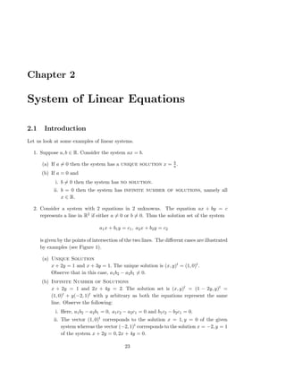
Definition 1.2.1 (Transpose of a Matrix). The transpose of an m × n matrix A = [aij] is
defined as the n × m matrix B = [bij], with bij = aji for 1 ≤ i ≤ m and 1 ≤ j ≤ n. The
transpose of A is denoted by At.
That is, if A =
1 4 5
0 1 2
then At =
1 0
4 1
5 2
. Thus, the transpose of a row vector is a
column vector and vice-versa.
Theorem 1.2.2. For any matrix A, (At)t = A.
Proof. Let A = [aij], At = [bij] and (At)t = [cij]. Then, the definition of transpose gives
cij = bji = aij for all i, j
and the result follows.
Definition 1.2.3 (Addition of Matrices). let A = [aij] and B = [bij] be two m×n matrices.
Then the sum A + B is defined to be the matrix C = [cij] with cij = aij + bij.
Note that, we define the sum of two matrices only when the order of the two matrices
are same.
Definition 1.2.4 (Multiplying a Scalar to a Matrix). Let A = [aij] be an m × n matrix.
Then for any element k ∈ R, we define kA = [kaij].
For example, if A =
1 4 5
0 1 2
and k = 5, then 5A =
5 20 25
0 5 10
.
Theorem 1.2.5. Let A, B and C be matrices of order m × n, and let k, ℓ ∈ R. Then
1. A + B = B + A (commutativity).
2. (A + B) + C = A + (B + C) (associativity).
3. k(ℓA) = (kℓ)A.
4. (k + ℓ)A = kA + ℓA.
Proof. Part 1.
Let A = [aij] and B = [bij]. Then
A + B = [aij] + [bij] = [aij + bij] = [bij + aij] = [bij] + [aij] = B + A
as real numbers commute.
The reader is required to prove the other parts as all the results follow from the prop-
erties of real numbers.](https://image.slidesharecdn.com/booklinear-160914134339/85/Book-linear-7-320.jpg)
![8 CHAPTER 1. INTRODUCTION TO MATRICES
Definition 1.2.6 (Additive Inverse). Let A be an m × n matrix.
1. Then there exists a matrix B with A + B = 0. This matrix B is called the additive
inverse of A, and is denoted by −A = (−1)A.
2. Also, for the matrix 0m×n, A + 0 = 0 + A = A. Hence, the matrix 0m×n is called the
additive identity.
Exercise 1.2.7. 1. Find a 3 × 3 non-zero matrix A satisfying A = At.
2. Find a 3 × 3 non-zero matrix A such that At = −A.
3. Find the 3 × 3 matrix A = [aij] satisfying aij = 1 if i = j and 2 otherwise.
4. Find the 3 × 3 matrix A = [aij] satisfying aij = 1 if |i − j| ≤ 1 and 0 otherwise.
5. Find the 4 × 4 matrix A = [aij] satisfying aij = i + j.
6. Find the 4 × 4 matrix A = [aij] satisfying aij = 2i+j.
7. Suppose A + B = A. Then show that B = 0.
8. Suppose A + B = 0. Then show that B = (−1)A = [−aij].
9. Let A =
1 −1
2 3
0 1
and B =
2 3 −1
1 1 2
. Compute A + Bt and B + At.
1.2.1 Multiplication of Matrices
Definition 1.2.8 (Matrix Multiplication / Product). Let A = [aij] be an m × n matrix
and B = [bij] be an n × r matrix. The product AB is a matrix C = [cij] of order m × r,
with
cij =
n
k=1
aikbkj = ai1b1j + ai2b2j + · · · + ainbnj.
That is, if Am×n =
· · · · · · · · · · · ·
· · · · · · · · · · · ·
ai1 ai2 · · · ain
· · · · · · · · · · · ·
· · · · · · · · · · · ·
and Bn×r =
... b1j
...
... b2j
...
...
...
...
... bmj
...
then
AB = [(AB)ij]m×r and (AB)ij = ai1b1j + ai2b2j + · · · + ainbnj.
Observe that the product AB is defined if and only if
the number of columns of A = the number of rows of B.](https://image.slidesharecdn.com/booklinear-160914134339/85/Book-linear-8-320.jpg)
![1.2. OPERATIONS ON MATRICES 9
For example, if A =
a b c
d e f
and B =
α β γ δ
x y z t
u v w s
then
AB =
aα + bx + cu aβ + by + cv aγ + bz + cw aδ + bt + cs
dα + ex + fu dβ + ey + fv dγ + ez + fw dδ + et + fs
. (1.2.1)
Observe that in Equation (1.2.1), the first row of AB can be re-written as
a · α β γ δ + b · x y z t + c · u v w s .
That is, if Rowi(B) denotes the i-th row of B for 1 ≤ i ≤ 3, then the matrix product AB
can be re-written as
AB =
a · Row1(B) + b · Row2(B) + c · Row3(B)
d · Row1(B) + e · Row2(B) + f · Row3(B)
. (1.2.2)
Similarly, observe that if Colj(A) denotes the j-th column of A for 1 ≤ j ≤ 3, then the
matrix product AB can be re-written as
AB = Col1(A) · α + Col2(A) · x + Col3(A) · u,
Col1(A) · β + Col2(A) · y + Col3(A) · v,
Col1(A) · γ + Col2(A) · z + Col3(A) · w
Col1(A) · δ + Col2(A) · t + Col3(A) · s] . (1.2.3)
Remark 1.2.9. Observe the following:
1. In this example, while AB is defined, the product BA is not defined.
However, for square matrices A and B of the same order, both the product AB and
BA are defined.
2. The product AB corresponds to operating on the rows of the matrix B (see Equa-
tion (1.2.2)). This is row method for calculating the matrix product.
3. The product AB also corresponds to operating on the columns of the matrix A (see
Equation (1.2.3)). This is column method for calculating the matrix product.
4. Let A = [aij] and B = [bij] be two matrices. Suppose a1, a2, . . . , an are the rows
of A and b1, b2, . . . , bp are the columns of B. If the product AB is defined, then
check that
AB = [Ab1, Ab2, . . . , Abp] =
a1B
a2B
...
anB
.](https://image.slidesharecdn.com/booklinear-160914134339/85/Book-linear-9-320.jpg)
![10 CHAPTER 1. INTRODUCTION TO MATRICES
Example 1.2.10. Let A =
1 2 0
1 0 1
0 −1 1
and B =
1 0 −1
0 0 1
0 −1 1
. Use the row/column
method of matrix multiplication to
1. find the second row of the matrix AB.
Solution: Observe that the second row of AB is obtained by multiplying the second
row of A with B. Hence, the second row of AB is
1 · [1, 0, −1] + 0 · [0, 0, 1] + 1 · [0, −1, 1] = [1, −1, 0].
2. find the third column of the matrix AB.
Solution: Observe that the third column of AB is obtained by multiplying A with
the third column of B. Hence, the third column of AB is
−1 ·
1
1
0
+ 1 ·
2
0
−1
+ 1 ·
0
1
1
=
1
0
0
.
Definition 1.2.11 (Commutativity of Matrix Product). Two square matrices A and B
are said to commute if AB = BA.
Remark 1.2.12. Note that if A is a square matrix of order n and if B is a scalar matrix of
order n then AB = BA. In general, the matrix product is not commutative. For example,
consider A =
1 1
0 0
and B =
1 0
1 0
. Then check that the matrix product
AB =
2 0
0 0
=
1 1
1 1
= BA.
Theorem 1.2.13. Suppose that the matrices A, B and C are so chosen that the matrix
multiplications are defined.
1. Then (AB)C = A(BC). That is, the matrix multiplication is associative.
2. For any k ∈ R, (kA)B = k(AB) = A(kB).
3. Then A(B + C) = AB + AC. That is, multiplication distributes over addition.
4. If A is an n × n matrix then AIn = InA = A.
5. For any square matrix A of order n and D = diag(d1, d2, . . . , dn), we have
• the first row of DA is d1 times the first row of A;
• for 1 ≤ i ≤ n, the ith row of DA is di times the ith row of A.
A similar statement holds for the columns of A when A is multiplied on the right by
D.](https://image.slidesharecdn.com/booklinear-160914134339/85/Book-linear-10-320.jpg)
![1.2. OPERATIONS ON MATRICES 11
Proof. Part 1. Let A = [aij]m×n, B = [bij]n×p and C = [cij]p×q. Then
(BC)kj =
p
ℓ=1
bkℓcℓj and (AB)iℓ =
n
k=1
aikbkℓ.
Therefore,
A(BC) ij
=
n
k=1
aik BC kj
=
n
k=1
aik
p
ℓ=1
bkℓcℓj
=
n
k=1
p
ℓ=1
aik bkℓcℓj =
n
k=1
p
ℓ=1
aikbkℓ cℓj
=
p
ℓ=1
n
k=1
aikbkℓ cℓj =
t
ℓ=1
AB iℓ
cℓj
= (AB)C ij
.
Part 5. For all j = 1, 2, . . . , n, we have
(DA)ij =
n
k=1
dikakj = diaij
as dik = 0 whenever i = k. Hence, the required result follows.
The reader is required to prove the other parts.
Exercise 1.2.14. 1. Find a 2 × 2 non-zero matrix A satisfying A2 = 0.
2. Find a 2 × 2 non-zero matrix A satisfying A2 = A and A = I2.
3. Find 2 × 2 non-zero matrices A, B and C satisfying AB = AC but B = C. That is,
the cancelation law doesn’t hold.
4. Let A =
0 1 0
0 0 1
1 0 0
. Compute A + 3A2 − A3 and aA3 + bA + cA2.
5. Let A and B be two matrices. If the matrix addition A + B is defined, then prove
that (A + B)t = At + Bt. Also, if the matrix product AB is defined then prove that
(AB)t = BtAt.
6. Let A = [a1, a2, . . . , an] and Bt = [b1, b2, . . . , bn]. Then check that order of AB is
1 × 1, whereas BA has order n × n. Determine the matrix products AB and BA.
7. Let A and B be two matrices such that the matrix product AB is defined.
(a) If the first row of A consists entirely of zeros, prove that the first row of AB
also consists entirely of zeros.
(b) If the first column of B consists entirely of zeros, prove that the first column of
AB also consists entirely of zeros.](https://image.slidesharecdn.com/booklinear-160914134339/85/Book-linear-11-320.jpg)

![1.2. OPERATIONS ON MATRICES 13
1.2.2 Inverse of a Matrix
Definition 1.2.15 (Inverse of a Matrix). Let A be a square matrix of order n.
1. A square matrix B is said to be a left inverse of A if BA = In.
2. A square matrix C is called a right inverse of A, if AC = In.
3. A matrix A is said to be invertible (or is said to have an inverse) if there exists
a matrix B such that AB = BA = In.
Lemma 1.2.16. Let A be an n × n matrix. Suppose that there exist n × n matrices B and
C such that AB = In and CA = In, then B = C.
Proof. Note that
C = CIn = C(AB) = (CA)B = InB = B.
Remark 1.2.17. 1. From the above lemma, we observe that if a matrix A is invertible,
then the inverse is unique.
2. As the inverse of a matrix A is unique, we denote it by A−1. That is, AA−1 =
A−1A = I.
Example 1.2.18. 1. Let A =
a b
c d
.
(a) If ad − bc = 0. Then verify that A−1 = 1
ad−bc
d −b
−c a
.
(b) If ad−bc = 0 then prove that either [a b] = α[c d] for some α ∈ R or [a c] = β[b d]
for some β ∈ R. Hence, prove that A is not invertible.
(c) In particular, the inverse of
2 3
4 7
equals 1
2
7 −3
−4 2
. Also, the matrices
1 2
0 0
,
1 0
4 0
and
4 2
6 3
do not have inverses.
2. Let A =
1 2 3
2 3 4
3 4 6
. Then A−1 =
−2 0 1
0 3 −2
1 −2 1
.
Theorem 1.2.19. Let A and B be two matrices with inverses A−1 and B−1, respectively.
Then
1. (A−1)−1 = A.
2. (AB)−1 = B−1A−1.
3. (At)−1 = (A−1)t.](https://image.slidesharecdn.com/booklinear-160914134339/85/Book-linear-13-320.jpg)
![14 CHAPTER 1. INTRODUCTION TO MATRICES
Proof. Proof of Part 1.
By definition AA−1 = A−1A = I. Hence, if we denote A−1 by B, then we get AB = BA = I.
Thus, the definition, implies B−1 = A, or equivalently (A−1)−1 = A.
Proof of Part 2.
Verify that (AB)(B−1A−1) = I = (B−1A−1)(AB).
Proof of Part 3.
We know AA−1 = A−1A = I. Taking transpose, we get
(AA−1
)t
= (A−1
A)t
= It
⇐⇒ (A−1
)t
At
= At
(A−1
)t
= I.
Hence, by definition (At)−1 = (A−1)t.
We will again come back to the study of invertible matrices in Sections 2.2 and 2.5.
Exercise 1.2.20. 1. Let A be an invertible matrix and let r be a positive integer. Prove
that (A−1)r = A−r.
2. Find the inverse of
− cos(θ) sin(θ)
sin(θ) cos(θ)
and
cos(θ) sin(θ)
− sin(θ) cos(θ)
.
3. Let A1, A2, . . . , Ar be invertible matrices. Prove that the product A1A2 · · · Ar is also
an invertible matrix.
4. Let xt = [1, 2, 3] and yt = [2, −1, 4]. Prove that xyt is not invertible even though xty
is invertible.
5. Let A be an n × n invertible matrix. Then prove that
(a) A cannot have a row or column consisting entirely of zeros.
(b) any two rows of A cannot be equal.
(c) any two columns of A cannot be equal.
(d) the third row of A cannot be equal to the sum of the first two rows, whenever
n ≥ 3.
(e) the third column of A cannot be equal to the first column minus the second
column, whenever n ≥ 3.
6. Suppose A is a 2 × 2 matrix satisfying (I + 3A)−1 =
1 2
2 1
. Determine the matrix
A.
7. Let A be a 3×3 matrix such that (I −A)−1 =
−2 0 1
0 3 −2
1 −2 1
. Determine the matrix
A [Hint: See Example 1.2.18.2 and Theorem 1.2.19.1].
8. Let A be a square matrix satisfying A3 + A − 2I = 0. Prove that A−1 = 1
2 A2 + I .
9. Let A = [aij] be an invertible matrix and let p be a nonzero real number. Then
determine the inverse of the matrix B = [pi−jaij].](https://image.slidesharecdn.com/booklinear-160914134339/85/Book-linear-14-320.jpg)
![1.3. SOME MORE SPECIAL MATRICES 15
1.3 Some More Special Matrices
Definition 1.3.1. 1. A matrix A over R is called symmetric if At = A and skew-
symmetric if At = −A.
2. A matrix A is said to be orthogonal if AAt = AtA = I.
Example 1.3.2. 1. Let A =
1 2 3
2 4 −1
3 −1 4
and B =
0 1 2
−1 0 −3
−2 3 0
. Then A is a
symmetric matrix and B is a skew-symmetric matrix.
2. Let A =
1√
3
1√
3
1√
3
1√
2
− 1√
2
0
1√
6
1√
6
− 2√
6
. Then A is an orthogonal matrix.
3. Let A = [aij] be an n × n matrix with aij equal to 1 if i − j = 1 and 0, otherwise.
Then An = 0 and Aℓ = 0 for 1 ≤ ℓ ≤ n − 1. The matrices A for which a positive
integer k exists such that Ak = 0 are called nilpotent matrices. The least positive
integer k for which Ak = 0 is called the order of nilpotency.
4. Let A =
1
2
1
2
1
2
1
2
. Then A2 = A. The matrices that satisfy the condition that A2 = A
are called idempotent matrices.
Exercise 1.3.3. 1. Let A be a real square matrix. Then S = 1
2(A + At) is symmetric,
T = 1
2(A − At) is skew-symmetric, and A = S + T.
2. Show that the product of two lower triangular matrices is a lower triangular matrix.
A similar statement holds for upper triangular matrices.
3. Let A and B be symmetric matrices. Show that AB is symmetric if and only if
AB = BA.
4. Show that the diagonal entries of a skew-symmetric matrix are zero.
5. Let A, B be skew-symmetric matrices with AB = BA. Is the matrix AB symmetric
or skew-symmetric?
6. Let A be a symmetric matrix of order n with A2 = 0. Is it necessarily true that
A = 0?
7. Let A be a nilpotent matrix. Prove that there exists a matrix B such that B(I +A) =
I = (I + A)B [ Hint: If Ak = 0 then look at I − A + A2 − · · · + (−1)k−1Ak−1].](https://image.slidesharecdn.com/booklinear-160914134339/85/Book-linear-15-320.jpg)
![16 CHAPTER 1. INTRODUCTION TO MATRICES
1.3.1 Submatrix of a Matrix
Definition 1.3.4. A matrix obtained by deleting some of the rows and/or columns of a
matrix is said to be a submatrix of the given matrix.
For example, if A =
1 4 5
0 1 2
, a few submatrices of A are
[1], [2],
1
0
, [1 5],
1 5
0 2
, A.
But the matrices
1 4
1 0
and
1 4
0 2
are not submatrices of A. (The reader is advised
to give reasons.)
Let A be an n × m matrix and B be an m × p matrix. Suppose r < m. Then, we can
decompose the matrices A and B as A = [P Q] and B =
H
K
; where P has order n × r
and H has order r × p. That is, the matrices P and Q are submatrices of A and P consists
of the first r columns of A and Q consists of the last m − r columns of A. Similarly, H
and K are submatrices of B and H consists of the first r rows of B and K consists of the
last m − r rows of B. We now prove the following important theorem.
Theorem 1.3.5. Let A = [aij] = [P Q] and B = [bij] =
H
K
be defined as above. Then
AB = PH + QK.
Proof. First note that the matrices PH and QK are each of order n × p. The matrix
products PH and QK are valid as the order of the matrices P, H, Q and K are respectively,
n × r, r × p, n × (m − r) and (m − r) × p. Let P = [Pij], Q = [Qij], H = [Hij], and
K = [kij]. Then, for 1 ≤ i ≤ n and 1 ≤ j ≤ p, we have
(AB)ij =
m
k=1
aikbkj =
r
k=1
aikbkj +
m
k=r+1
aikbkj
=
r
k=1
PikHkj +
m
k=r+1
QikKkj
= (PH)ij + (QK)ij = (PH + QK)ij.
Remark 1.3.6. Theorem 1.3.5 is very useful due to the following reasons:
1. The order of the matrices P, Q, H and K are smaller than that of A or B.
2. It may be possible to block the matrix in such a way that a few blocks are either
identity matrices or zero matrices. In this case, it may be easy to handle the matrix
product using the block form.](https://image.slidesharecdn.com/booklinear-160914134339/85/Book-linear-16-320.jpg)
![1.3. SOME MORE SPECIAL MATRICES 17
3. Or when we want to prove results using induction, then we may assume the result for
r × r submatrices and then look for (r + 1) × (r + 1) submatrices, etc.
For example, if A =
1 2 0
2 5 0
and B =
a b
c d
e f
, Then
AB =
1 2
2 5
a b
c d
+
0
0
[e f] =
a + 2c b + 2d
2a + 5c 2b + 5d
.
If A =
0 −1 2
3 1 4
−2 5 −3
, then A can be decomposed as follows:
A =
0 −1 2
3 1 4
−2 5 −3
, or A =
0 −1 2
3 1 4
−2 5 −3
, or
A =
0 −1 2
3 1 4
−2 5 −3
and so on.
Suppose A =
m1 m2
n1
n2
P Q
R S
and B =
s1 s2
r1
r2
E F
G H
. Then the matrices P, Q, R, S
and E, F, G, H, are called the blocks of the matrices A and B, respectively.
Even if A+B is defined, the orders of P and E may not be same and hence, we may
not be able to add A and B in the block form. But, if A + B and P + E is defined then
A + B =
P + E Q + F
R + G S + H
.
Similarly, if the product AB is defined, the product PE need not be defined. Therefore,
we can talk of matrix product AB as block product of matrices, if both the products AB
and PE are defined. And in this case, we have AB =
PE + QG PF + QH
RE + SG RF + SH
.
That is, once a partition of A is fixed, the partition of B has to be properly
chosen for purposes of block addition or multiplication.
Exercise 1.3.7. 1. Complete the proofs of Theorems 1.2.5 and 1.2.13.
2. Let A =
1/2 0 0
0 1 0
0 0 1
, B =
1 0 0
−2 1 0
−3 0 1
and C =
2 2 2 6
2 1 2 5
3 3 4 10
. Compute
(a) the first row of AC,
(b) the first row of B(AC),](https://image.slidesharecdn.com/booklinear-160914134339/85/Book-linear-17-320.jpg)
![18 CHAPTER 1. INTRODUCTION TO MATRICES
(c) the second row of B(AC), and
(d) the third row of B(AC).
(e) Let xt = [1, 1, 1, −1]. Compute the matrix product Cx.
3. Let x =
x1
x2
and y =
y1
y2
. Determine the 2 × 2 matrix
(a) A such that the y = Ax gives rise to counter-clockwise rotation through an angle
α.
(b) B such that y = Bx gives rise to the reflection along the line y = (tan γ)x.
Now, let C and D be two 2× 2 matrices such that y = Cx gives rise to counter-
clockwise rotation through an angle β and y = Dx gives rise to the reflection
along the line y = (tan δ) x, respectively. Then prove that
(c) y = (AC)x or y = (CA)x give rise to counter-clockwise rotation through an
angle α + β.
(d) y = (BD)x or y = (DB)x give rise to rotations. Which angles do they repre-
sent?
(e) What can you say about y = (AB)x or y = (BA)x ?
4. Let A =
1 0
0 −1
, B =
cos α − sin α
sin α cos α
and C =
cos θ − sin θ
sin θ cos θ
. If x =
x1
x2
and y =
y1
y2
then geometrically interpret the following:
(a) y = Ax, y = Bx and y = Cx.
(b) y = (BC)x, y = (CB)x, y = (BA)x and y = (AB)x.
5. Consider the two coordinate transformations
x1 = a11y1 + a12y2
x2 = a21y1 + a22y2
and
y1 = b11z1 + b12z2
y2 = b21z1 + b22z2
.
(a) Compose the two transformations to express x1, x2 in terms of z1, z2.
(b) If xt = [x1, x2], yt = [y1, y2] and zt = [z1, z2] then find matrices A, B and C
such that x = Ay, y = Bz and x = Cz.
(c) Is C = AB?
6. Let A be an n × n matrix. Then trace of A, denoted tr(A), is defined as
tr(A) = a11 + a22 + · · · ann.
(a) Let A =
3 2
2 2
and B =
4 −3
−5 1
. Compute tr(A) and tr(B).](https://image.slidesharecdn.com/booklinear-160914134339/85/Book-linear-18-320.jpg)
![20 CHAPTER 1. INTRODUCTION TO MATRICES
13. Let x be an n × 1 matrix satisfying xtx = 1.
(a) Define A = In − 2xxt. Prove that A is symmetric and A2 = I. The matrix A
is commonly known as the Householder matrix.
(b) Let α = 1 be a real number and define A = In −αxxt. Prove that A is symmetric
and invertible [Hint: the inverse is also of the form In + βxxt for some value of
β].
14. Let A be an n × n invertible matrix and let x and y be two n × 1 matrices. Also,
let β be a real number such that α = 1 + βytA−1x = 0. Then prove the famous
Shermon-Morrison formula
(A + βxyt
)−1
= A−1
−
β
α
A−1
xyt
A−1
.
This formula gives the information about the inverse when an invertible matrix is
modified by a rank one matrix.
15. Let J be an n × n matrix having each entry 1.
(a) Prove that J2 = nJ.
(b) Let α1, α2, β1, β2 ∈ R. Prove that there exist α3, β3 ∈ R such that
(α1In + β1J) · (α2In + β2J) = α3In + β3J.
(c) Let α, β ∈ R with α = 0 and α + nβ = 0 and define A = αIn + βJ. Prove that
A is invertible.
16. Let A be an upper triangular matrix. If A∗A = AA∗ then prove that A is a diagonal
matrix. The same holds for lower triangular matrix.
1.4 Summary
In this chapter, we started with the definition of a matrix and came across lots of examples.
In particular, the following examples were important:
1. The zero matrix of size m × n, denoted 0m×n or 0.
2. The identity matrix of size n × n, denoted In or I.
3. Triangular matrices
4. Hermitian/Symmetric matrices
5. Skew-Hermitian/skew-symmetric matrices
6. Unitary/Orthogonal matrices
We also learnt product of two matrices. Even though it seemed complicated, it basically
tells the following:](https://image.slidesharecdn.com/booklinear-160914134339/85/Book-linear-20-320.jpg)


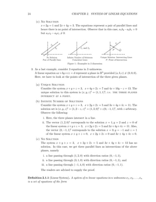
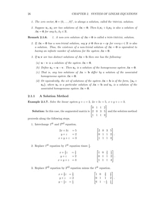
![2.1. INTRODUCTION 25
a11x1 + a12x2 + · · · + a1nxn = b1
a21x1 + a22x2 + · · · + a2nxn = b2
...
... (2.1.1)
am1x1 + am2x2 + · · · + amnxn = bm
where for 1 ≤ i ≤ n, and 1 ≤ j ≤ m; aij, bi ∈ R. Linear System (2.1.1) is called homoge-
neous if b1 = 0 = b2 = · · · = bm and non-homogeneous otherwise.
We rewrite the above equations in the form Ax = b, where
A =
a11 a12 · · · a1n
a21 a22 · · · a2n
...
...
...
...
am1 am2 · · · amn
, x =
x1
x2
...
xn
, and b =
b1
b2
...
bm
The matrix A is called the coefficient matrix and the block matrix [A b] , is called
the augmented matrix of the linear system (2.1.1).
Remark 2.1.2. 1. The first column of the augmented matrix corresponds to the coeffi-
cients of the variable x1.
2. In general, the jth column of the augmented matrix corresponds to the coefficients of
the variable xj, for j = 1, 2, . . . , n.
3. The (n + 1)th column of the augmented matrix consists of the vector b.
4. The ith row of the augmented matrix represents the ith equation for i = 1, 2, . . . , m.
That is, for i = 1, 2, . . . , m and j = 1, 2, . . . , n, the entry aij of the coefficient matrix
A corresponds to the ith linear equation and the jth variable xj.
Definition 2.1.3. For a system of linear equations Ax = b, the system Ax = 0 is called
the associated homogeneous system.
Definition 2.1.4 (Solution of a Linear System). A solution of Ax = b is a column vector
y with entries y1, y2, . . . , yn such that the linear system (2.1.1) is satisfied by substituting
yi in place of xi. The collection of all solutions is called the solution set of the system.
That is, if yt = [y1, y2, . . . , yn] is a solution of the linear system Ax = b then Ay = b
holds. For example, from Example 3.3a, we see that the vector yt = [1, 1, 1] is a solution
of the system Ax = b, where A =
1 1 1
1 4 2
4 10 −1
, xt = [x, y, z] and bt = [3, 7, 13].
We now state a theorem about the solution set of a homogeneous system. The readers
are advised to supply the proof.
Theorem 2.1.5. Consider the homogeneous linear system Ax = 0. Then](https://image.slidesharecdn.com/booklinear-160914134339/85/Book-linear-25-320.jpg)
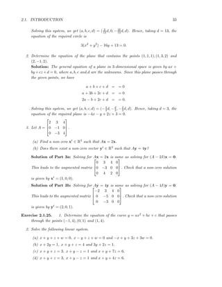
![2.1. INTRODUCTION 27
4. Replace 3rd equation by 3rd equation minus the 2nd equation.
x + 3
2z = 5
2
y + z = 2
−3
2z = −3
2
1 0 3
2
5
2
0 1 1 2
0 0 −3
2 −3
2
.
5. Replace 3rd equation by 3rd equation times −2
3 .
x + 3
2z = 5
2
y + z = 2
z = 1
1 0 3
2
5
2
0 1 1 2
0 0 1 1
.
The last equation gives z = 1. Using this, the second equation gives y = 1. Finally,
the first equation gives x = 1. Hence the solution set is {(x, y, z)t : (x, y, z) = (1, 1, 1)}, a
unique solution.
In Example 2.1.7, observe that certain operations on equations (rows of the augmented
matrix) helped us in getting a system in Item 5, which was easily solvable. We use this
idea to define elementary row operations and equivalence of two linear systems.
Definition 2.1.8 (Elementary Row Operations). Let A be an m × n matrix. Then the
elementary row operations are defined as follows:
1. Rij: Interchange of the ith and the jth row of A.
2. For c = 0, Rk(c): Multiply the kth row of A by c.
3. For c = 0, Rij(c): Replace the jth row of A by the jth row of A plus c times the ith
row of A.
Definition 2.1.9 (Equivalent Linear Systems). Let [A b] and [C d] be augmented ma-
trices of two linear systems. Then the two linear systems are said to be equivalent if [C d]
can be obtained from [A b] by application of a finite number of elementary row operations.
Definition 2.1.10 (Row Equivalent Matrices). Two matrices are said to be row-equivalent
if one can be obtained from the other by a finite number of elementary row operations.
Thus, note that linear systems at each step in Example 2.1.7 are equivalent to each
other. We also prove the following result that relates elementary row operations with the
solution set of a linear system.
Lemma 2.1.11. Let Cx = d be the linear system obtained from Ax = b by application of
a single elementary row operation. Then Ax = b and Cx = d have the same solution set.
Proof. We prove the result for the elementary row operation Rjk(c) with c = 0. The reader
is advised to prove the result for other elementary operations.](https://image.slidesharecdn.com/booklinear-160914134339/85/Book-linear-27-320.jpg)
![28 CHAPTER 2. SYSTEM OF LINEAR EQUATIONS
In this case, the systems Ax = b and Cx = d vary only in the kth equation. Let
(α1, α2, . . . , αn) be a solution of the linear system Ax = b. Then substituting for αi’s in
place of xi’s in the kth and jth equations, we get
ak1α1 + ak2α2 + · · · aknαn = bk, and aj1α1 + aj2α2 + · · · ajnαn = bj.
Therefore,
(ak1 + caj1)α1 + (ak2 + caj2)α2 + · · · + (akn + cajn)αn = bk + cbj. (2.1.2)
But then the kth equation of the linear system Cx = d is
(ak1 + caj1)x1 + (ak2 + caj2)x2 + · · · + (akn + cajn)xn = bk + cbj. (2.1.3)
Therefore, using Equation (2.1.2), (α1, α2, . . . , αn) is also a solution for kth Equation
(2.1.3).
Use a similar argument to show that if (β1, β2, . . . , βn) is a solution of the linear system
Cx = d then it is also a solution of the linear system Ax = b. Hence, the required result
follows.
The readers are advised to use Lemma 2.1.11 as an induction step to prove the main
result of this subsection which is stated next.
Theorem 2.1.12. Two equivalent linear systems have the same solution set.
2.1.2 Gauss Elimination Method
We first define the Gauss elimination method and give a few examples to understand the
method.
Definition 2.1.13 (Forward/Gauss Elimination Method). The Gaussian elimination method
is a procedure for solving a linear system Ax = b (consisting of m equations in n unknowns)
by bringing the augmented matrix
[A b] =
a11 a12 · · · a1m · · · a1n b1
a21 a22 · · · a2m · · · a2n b2
...
...
...
...
...
...
am1 am2 · · · amm · · · amn bm
to an upper triangular form
c11 c12 · · · c1m · · · c1n d1
0 c22 · · · c2m · · · c2n d2
...
...
...
...
...
...
0 0 · · · cmm · · · cmn dm
by application of elementary row operations. This elimination process is also called the
forward elimination method.](https://image.slidesharecdn.com/booklinear-160914134339/85/Book-linear-28-320.jpg)
![2.1. INTRODUCTION 29
We have already seen an example before defining the notion of row equivalence. We
give two more examples to illustrate the Gauss elimination method.
Example 2.1.14. Solve the following linear system by Gauss elimination method.
x + y + z = 3, x + 2y + 2z = 5, 3x + 4y + 4z = 11
Solution: Let A =
1 1 1
1 2 2
3 4 4
and b =
3
5
11
. The Gauss Elimination method starts
with the augmented matrix [A b] and proceeds as follows:
1. Replace 2nd equation by 2nd equation minus the 1st equation.
x + y + z = 3
y + z = 2
3x + 4y + 4z = 11
1 1 1 3
0 1 1 2
3 4 4 11
.
2. Replace 3rd equation by 3rd equation minus 3 times 1st equation.
x + y + z = 3
y + z = 2
y + z = 2
1 1 1 3
0 1 1 2
0 1 1 2
.
3. Replace 3rd equation by 3rd equation minus the 2nd equation.
x + y + z = 3
y + z = 2
1 1 1 3
0 1 1 2
0 0 0 0
.
Thus, the solution set is {(x, y, z)t : (x, y, z) = (1, 2 − z, z)} or equivalently {(x, y, z)t :
(x, y, z) = (1, 2, 0)+z(0, −1, 1)}, with z arbitrary. In other words, the system has infinite
number of solutions. Observe that the vector yt = (1, 2, 0) satisfies Ay = b and the
vector zt = (0, −1, 1) is a solution of the homogeneous system Ax = 0.
Example 2.1.15. Solve the following linear system by Gauss elimination method.
x + y + z = 3, x + 2y + 2z = 5, 3x + 4y + 4z = 12
Solution: Let A =
1 1 1
1 2 2
3 4 4
and b =
3
5
12
. The Gauss Elimination method starts
with the augmented matrix [A b] and proceeds as follows:
1. Replace 2nd equation by 2nd equation minus the 1st equation.
x + y + z = 3
y + z = 2
3x + 4y + 4z = 12
1 1 1 3
0 1 1 2
3 4 4 12
.](https://image.slidesharecdn.com/booklinear-160914134339/85/Book-linear-29-320.jpg)
![30 CHAPTER 2. SYSTEM OF LINEAR EQUATIONS
2. Replace 3rd equation by 3rd equation minus 3 times 1st equation.
x + y + z = 3
y + z = 2
y + z = 3
1 1 1 3
0 1 1 2
0 1 1 3
.
3. Replace 3rd equation by 3rd equation minus the 2nd equation.
x + y + z = 3
y + z = 2
0 = 1
1 1 1 3
0 1 1 2
0 0 0 1
.
The third equation in the last step is
0x + 0y + 0z = 1.
This can never hold for any value of x, y, z. Hence, the system has no solution.
Remark 2.1.16. Note that to solve a linear system Ax = b, one needs to apply only the
row operations to the augmented matrix [A b].
Definition 2.1.17 (Row Echelon Form of a Matrix). A matrix C is said to be in the row
echelon form if
1. the rows consisting entirely of zeros appears after the non-zero rows,
2. the first non-zero entry in a non-zero row is 1. This term is called the leading term
or a leading 1. The column containing this term is called the leading column.
3. In any two successive non-zero rows, the leading 1 in the lower row occurs farther to
the right than the leading 1 in the higher row.
Example 2.1.18. The matrices
0 1 4 2
0 0 1 1
0 0 0 0
and
1 1 0 2 3
0 0 0 1 4
0 0 0 0 1
are in
row-echelon form. Whereas, the matrices
0 1 4 2
0 0 0 0
0 0 1 1
,
1 1 0 2 3
0 0 0 1 4
0 0 0 0 2
and
1 1 0 2 3
0 0 0 0 1
0 0 0 1 4
are not in row-echelon form.
Definition 2.1.19 (Basic, Free Variables). Let Ax = b be a linear system consisting of
m equations in n unknowns. Suppose the application of Gauss elimination method to the
augmented matrix [A b] yields the matrix [C d].
1. Then the variables corresponding to the leading columns (in the first n columns of
[C d]) are called the basic variables.](https://image.slidesharecdn.com/booklinear-160914134339/85/Book-linear-30-320.jpg)
![2.1. INTRODUCTION 31
2. The variables which are not basic are called free variables.
The free variables are called so as they can be assigned arbitrary values. Also, the basic
variables can be written in terms of the free variables and hence the value of basic variables
in the solution set depend on the values of the free variables.
Remark 2.1.20. Observe the following:
1. In Example 2.1.14, the solution set was given by
(x, y, z) = (1, 2 − z, z) = (1, 2, 0) + z(0, −1, 1), with z arbitrary.
That is, we had x, y as two basic variables and z as a free variable.
2. Example 2.1.15 didn’t have any solution because the row-echelon form of the aug-
mented matrix had a row of the form [0, 0, 0, 1].
3. Suppose the application of row operations to [A b] yields the matrix [C d] which
is in row echelon form. If [C d] has r non-zero rows then [C d] will consist of r
leading terms or r leading columns. Therefore, the linear system Ax = b will
have r basic variables and n − r free variables.
Before proceeding further, we have the following definition.
Definition 2.1.21 (Consistent, Inconsistent). A linear system is called consistent if it
admits a solution and is called inconsistent if it admits no solution.
We are now ready to prove conditions under which the linear system Ax = b is consis-
tent or inconsistent.
Theorem 2.1.22. Consider the linear system Ax = b, where A is an m × n matrix
and xt = (x1, x2, . . . , xn). If one obtains [C d] as the row-echelon form of [A b] with
dt = (d1, d2, . . . , dm) then
1. Ax = b is inconsistent (has no solution) if [C d] has a row of the form [0t 1], where
0t = (0, . . . , 0).
2. Ax = b is consistent (has a solution) if [C d] has no row of the form [0t 1].
Furthermore,
(a) if the number of variables equals the number of leading terms then Ax = b has
a unique solution.
(b) if the number of variables is strictly greater than the number of leading terms
then Ax = b has infinite number of solutions.
Proof. Part 1: The linear equation corresponding to the row [0t 1] equals
0x1 + 0x2 + · · · + 0xn = 1.](https://image.slidesharecdn.com/booklinear-160914134339/85/Book-linear-31-320.jpg)
![32 CHAPTER 2. SYSTEM OF LINEAR EQUATIONS
Obviously, this equation has no solution and hence the system Cx = d has no solution.
Thus, by Theorem 2.1.12, Ax = b has no solution. That is, Ax = b is inconsistent.
Part 2: Suppose [C d] has r non-zero rows. As [C d] is in row echelon form there
exist positive integers 1 ≤ i1 < i2 < . . . < ir ≤ n such that entries cℓiℓ
for 1 ≤ ℓ ≤ r
are leading terms. This in turn implies that the variables xij , for 1 ≤ j ≤ r are the basic
variables and the remaining n − r variables, say xt1 , xt2 , . . . , xtn−r , are free variables. So
for each ℓ, 1 ≤ ℓ ≤ r, one obtains xiℓ
+
k>iℓ
cℓkxk = dℓ (k > iℓ in the summation as [C d]
is a matrix in the row reduced echelon form). Or equivalently,
xiℓ
= dℓ −
r
j=ℓ+1
cℓij
xij −
n−r
s=1
cℓts xts for 1 ≤ l ≤ r.
Hence, a solution of the system Cx = d is given by
xts = 0 for s = 1, . . . , n − r and xir = dr, xir−1 = dr−1 − dr, . . . , xi1 = d1 −
r
j=2
cℓij
dj.
Thus, by Theorem 2.1.12 the system Ax = b is consistent. In case of Part 2a, there are no
free variables and hence the unique solution is given by
xn = dn, xn−1 = dn−1 − dn, . . . , x1 = d1 −
n
j=2
cℓij
dj.
In case of Part 2b, there is at least one free variable and hence Ax = b has infinite number
of solutions. Thus, the proof of the theorem is complete.
We omit the proof of the next result as it directly follows from Theorem 2.1.22.
Corollary 2.1.23. Consider the homogeneous system Ax = 0. Then
1. Ax = 0 is always consistent as 0 is a solution.
2. If m < n then n−m > 0 and there will be at least n−m free variables. Thus Ax = 0
has infinite number of solutions. Or equivalently, Ax = 0 has a non-trivial solution.
We end this subsection with some applications related to geometry.
Example 2.1.24. 1. Determine the equation of the line/circle that passes through the
points (−1, 4), (0, 1) and (1, 4).
Solution: The general equation of a line/circle in 2-dimensional plane is given by
a(x2 + y2) + bx + cy + d = 0, where a, b, c and d are the unknowns. Since this curve
passes through the given points, we have
a((−1)2
+ 42
) + (−1)b + 4c + d = = 0
a((0)2
+ 12
) + (0)b + 1c + d = = 0
a((1)2
+ 42
) + (1)b + 4c + d = = 0.](https://image.slidesharecdn.com/booklinear-160914134339/85/Book-linear-32-320.jpg)
![34 CHAPTER 2. SYSTEM OF LINEAR EQUATIONS
(e) x + y + z = 3, x + y − z = 1, x + y + 4z = 6 and x + y − 4z = −1.
3. For what values of c and k, the following systems have i) no solution, ii) a unique
solution and iii) infinite number of solutions.
(a) x + y + z = 3, x + 2y + cz = 4, 2x + 3y + 2cz = k.
(b) x + y + z = 3, x + y + 2cz = 7, x + 2y + 3cz = k.
(c) x + y + 2z = 3, x + 2y + cz = 5, x + 2y + 4z = k.
(d) kx + y + z = 1, x + ky + z = 1, x + y + kz = 1.
(e) x + 2y − z = 1, 2x + 3y + kz = 3, x + ky + 3z = 2.
(f) x − 2y = 1, x − y + kz = 1, ky + 4z = 6.
4. For what values of a, does the following systems have i) no solution, ii) a unique
solution and iii) infinite number of solutions.
(a) x + 2y + 3z = 4, 2x + 5y + 5z = 6, 2x + (a2 − 6)z = a + 20.
(b) x + y + z = 3, 2x + 5y + 4z = a, 3x + (a2 − 8)z = 12.
5. Find the condition(s) on x, y, z so that the system of linear equations given below (in
the unknowns a, b and c) is consistent?
(a) a + 2b − 3c = x, 2a + 6b − 11c = y, a − 2b + 7c = z
(b) a + b + 5c = x, a + 3c = y, 2a − b + 4c = z
(c) a + 2b + 3c = x, 2a + 4b + 6c = y, 3a + 6b + 9c = z
6. Let A be an n×n matrix. If the system A2x = 0 has a non trivial solution then show
that Ax = 0 also has a non trivial solution.
7. Prove that we need to have 5 set of distinct points to specify a general conic in 2-
dimensional plane.
8. Let ut = (1, 1, −2) and vt = (−1, 2, 3). Find condition on x, y and z such that the
system cut + dvt = (x, y, z) in the unknowns c and d is consistent.
2.1.3 Gauss-Jordan Elimination
The Gauss-Jordan method consists of first applying the Gauss Elimination method to get
the row-echelon form of the matrix [A b] and then further applying the row operations
as follows. For example, consider Example 2.1.7. We start with Step 5 and apply row
operations once again. But this time, we start with the 3rd row.
I. Replace 2nd equation by 2nd equation minus the 3rd equation.
x + 3
2z = 5
2
y = 2
z = 1
1 0 3
2
5
2
0 1 0 1
0 0 1 1
.](https://image.slidesharecdn.com/booklinear-160914134339/85/Book-linear-34-320.jpg)
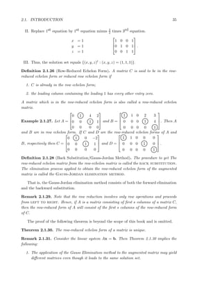
![36 CHAPTER 2. SYSTEM OF LINEAR EQUATIONS
2. The application of the Gauss-Jordan method to the augmented matrix yields the same
matrix and also the same solution set even though we may have used different sequence
of row operations.
Example 2.1.32. Consider Ax = b, where A is a 3 × 3 matrix. Let [C d] be the row-
reduced echelon form of [A b]. Also, assume that the first column of A has a non-zero
entry. Then the possible choices for the matrix [C d] with respective solution sets are given
below:
1.
1 0 0 d1
0 1 0 d2
0 0 1 d3
. Ax = b has a unique solution, (x, y, z) = (d1, d2, d3).
2.
1 0 α d1
0 1 β d2
0 0 0 1
,
1 α 0 d1
0 0 1 d2
0 0 0 1
or
1 α β d1
0 0 0 1
0 0 0 0
. Ax = b has no solution for
any choice of α, β.
3.
1 0 α d1
0 1 β d2
0 0 0 0
,
1 α 0 d1
0 0 1 d2
0 0 0 0
,
1 α β d1
0 0 0 0
0 0 0 0
. Ax = b has Infinite number
of solutions for every choice of α, β.
Exercise 2.1.33. 1. Let Ax = b be a linear system in 2 unknowns. What are the
possible choices for the row-reduced echelon form of the augmented matrix [A b]?
2. Find the row-reduced echelon form of the following matrices:
0 0 1
1 0 3
3 0 7
,
0 1 1 3
0 0 1 3
1 1 0 0
,
0 −1 1
−2 0 3
−5 1 0
,
−1 −1 −2 3
3 3 −3 −3
1 1 2 2
−1 −1 2 −2
.
3. Find all the solutions of the following system of equations using Gauss-Jordan method.
No other method will be accepted.
x + y – 2 u + v = 2
z + u + 2 v = 3
v + w = 3
v + 2 w = 5
2.2 Elementary Matrices
In the previous section, we solved a system of linear equations with the help of either the
Gauss Elimination method or the Gauss-Jordan method. These methods required us to
make row operations on the augmented matrix. Also, we know that (see Section 1.2.1 )](https://image.slidesharecdn.com/booklinear-160914134339/85/Book-linear-36-320.jpg)
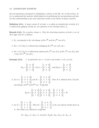
![38 CHAPTER 2. SYSTEM OF LINEAR EQUATIONS
Or equivalently, check that
E13A = A1 =
1 1 1 3
2 0 3 5
0 1 1 2
, E12(−2)A1 = A2 =
1 1 1 3
0 −2 1 −1
0 1 1 2
,
E23A2 = A3 =
1 1 1 3
0 1 1 2
0 −2 1 −1
, E23(2)A3 = A4 =
1 1 1 3
0 1 1 2
0 0 3 3
,
E3(1/3)A4 = A5 =
1 1 1 3
0 1 1 2
0 0 1 1
, E21(−1)A5 = A6 =
1 0 0 1
0 1 1 2
0 0 1 1
,
E32(−1)A6 = B =
1 0 0 1
0 1 0 1
0 0 1 1
.
Remark 2.2.4. Observe the following:
1. The inverse of the elementary matrix Eij is the matrix Eij itself. That is, EijEij =
I = EijEij.
2. Let c = 0. Then the inverse of the elementary matrix Ek(c) is the matrix Ek(1/c).
That is, Ek(c)Ek(1/c) = I = Ek(1/c)Ek(c).
3. Let c = 0. Then the inverse of the elementary matrix Eij(c) is the matrix Eij(−c).
That is, Eij(c)Eij(−c) = I = Eij(−c)Eij(c).
That is, all the elementary matrices are invertible and the inverses are also elemen-
tary matrices.
4. Suppose the row-reduced echelon form of the augmented matrix [A b] is the matrix
[C d]. As row operations correspond to multiplying on the left with elementary
matrices, we can find elementary matrices, say E1, E2, . . . , Ek, such that
Ek · Ek−1 · · · E2 · E1 · [A b] = [C d].
That is, the Gauss-Jordan method (or Gauss Elimination method) is equivalent to
multiplying by a finite number of elementary matrices on the left to [A b].
We are now ready to prove a equivalent statements in the study of invertible matrices.
Theorem 2.2.5. Let A be a square matrix of order n. Then the following statements are
equivalent.
1. A is invertible.
2. The homogeneous system Ax = 0 has only the trivial solution.
3. The row-reduced echelon form of A is In.](https://image.slidesharecdn.com/booklinear-160914134339/85/Book-linear-38-320.jpg)
![2.2. ELEMENTARY MATRICES 39
4. A is a product of elementary matrices.
Proof. 1 =⇒ 2
As A is invertible, we have A−1A = In = AA−1. Let x0 be a solution of the homoge-
neous system Ax = 0. Then, Ax0 = 0 and Thus, we see that 0 is the only solution of the
homogeneous system Ax = 0.
2 =⇒ 3
Let xt = [x1, x2, . . . , xn]. As 0 is the only solution of the linear system Ax = 0, the
final equations are x1 = 0, x2 = 0, . . . , xn = 0. These equations can be rewritten as
1 · x1 + 0 · x2 + 0 · x3 + · · · + 0 · xn = 0
0 · x1 + 1 · x2 + 0 · x3 + · · · + 0 · xn = 0
0 · x1 + 0 · x2 + 1 · x3 + · · · + 0 · xn = 0
... =
...
0 · x1 + 0 · x2 + 0 · x3 + · · · + 1 · xn = 0.
That is, the final system of homogeneous system is given by In · x = 0. Or equivalently,
the row-reduced echelon form of the augmented matrix [A 0] is [In 0]. That is, the
row-reduced echelon form of A is In.
3 =⇒ 4
Suppose that the row-reduced echelon form of A is In. Then using Remark 2.2.4.4,
there exist elementary matrices E1, E2, . . . , Ek such that
E1E2 · · · EkA = In. (2.2.4)
Now, using Remark 2.2.4, the matrix E−1
j is an elementary matrix and is the inverse of
Ej for 1 ≤ j ≤ k. Therefore, successively multiplying Equation (2.2.4) on the left by
E−1
1 , E−1
2 , . . . , E−1
k , we get
A = E−1
k E−1
k−1 · · · E−1
2 E−1
1
and thus A is a product of elementary matrices.
4 =⇒ 1
Suppose A = E1E2 · · · Ek; where the Ei’s are elementary matrices. As the elementary
matrices are invertible (see Remark 2.2.4) and the product of invertible matrices is also
invertible, we get the required result.
As an immediate consequence of Theorem 2.2.5, we have the following important result.
Theorem 2.2.6. Let A be a square matrix of order n.
1. Suppose there exists a matrix C such that CA = In. Then A−1 exists.
2. Suppose there exists a matrix B such that AB = In. Then A−1 exists.](https://image.slidesharecdn.com/booklinear-160914134339/85/Book-linear-39-320.jpg)
![40 CHAPTER 2. SYSTEM OF LINEAR EQUATIONS
Proof. Suppose there exists a matrix C such that CA = In. Let x0 be a solution of the
homogeneous system Ax = 0. Then Ax0 = 0 and
x0 = In · x0 = (CA)x0 = C(Ax0) = C0 = 0.
That is, the homogeneous system Ax = 0 has only the trivial solution. Hence, using
Theorem 2.2.5, the matrix A is invertible.
Using the first part, it is clear that the matrix B in the second part, is invertible. Hence
AB = In = BA.
Thus, A is invertible as well.
Remark 2.2.7. Theorem 2.2.6 implies the following:
1. “if we want to show that a square matrix A of order n is invertible, it is enough to
show the existence of
(a) either a matrix B such that AB = In
(b) or a matrix C such that CA = In.
2. Let A be an invertible matrix of order n. Suppose there exist elementary matrices
E1, E2, . . . , Ek such that E1E2 · · · EkA = In. Then A−1 = E1E2 · · · Ek.
Remark 2.2.7 gives the following method of computing the inverse of a matrix.
Summary: Let A be an n × n matrix. Apply the Gauss-Jordan method to the matrix
[A In]. Suppose the row-reduced echelon form of the matrix [A In] is [B C]. If B = In,
then A−1 = C or else A is not invertible.
Example 2.2.8. Find the inverse of the matrix
0 0 1
0 1 1
1 1 1
using the Gauss-Jordan method.
Solution: let us apply the Gauss-Jordan method to the matrix
0 0 1 1 0 0
0 1 1 0 1 0
1 1 1 0 0 1
.
1.
0 0 1 1 0 0
0 1 1 0 1 0
1 1 1 0 0 1
−−→
R13
1 1 1 0 0 1
0 1 1 0 1 0
0 0 1 1 0 0
2.
1 1 1 0 0 1
0 1 1 0 1 0
0 0 1 1 0 0
−−−−−→
R31(−1)
−−−−−→
R32(−1)
1 1 0 −1 0 1
0 1 0 −1 1 0
0 0 1 1 0 0
3.
1 1 0 −1 0 1
0 1 0 −1 1 0
0 0 1 1 0 0
−−−−−→
R21(−1)
1 0 0 0 −1 1
0 1 0 −1 1 0
0 0 1 1 0 0
.](https://image.slidesharecdn.com/booklinear-160914134339/85/Book-linear-40-320.jpg)
![2.2. ELEMENTARY MATRICES 41
Thus, the inverse of the given matrix is
0 −1 1
−1 1 0
1 0 0
.
Exercise 2.2.9. 1. Find the inverse of the following matrices using the Gauss-Jordan
method.
(i)
1 2 3
1 3 2
2 4 7
, (ii)
1 3 3
2 3 2
2 4 7
, (iii)
2 1 1
1 2 1
1 1 2
, (iv)
0 0 2
0 2 1
2 1 1
.
2. Which of the following matrices are elementary?
2 0 1
0 1 0
0 0 1
,
1
2 0 0
0 1 0
0 0 1
,
1 −1 0
0 1 0
0 0 1
,
1 0 0
5 1 0
0 0 1
,
0 0 1
0 1 0
1 0 0
,
0 0 1
1 0 0
0 1 0
.
3. Let A =
2 1
1 2
. Find the elementary matrices E1, E2, E3 and E4 such that E4 · E3 ·
E2 · E1 · A = I2.
4. Let B =
1 1 1
0 1 1
0 0 3
. Determine elementary matrices E1, E2 and E3 such that E3 ·
E2 · E1 · B = I3.
5. In Exercise 2.2.9.3, let C = E4 · E3 · E2 · E1. Then check that AC = I2.
6. In Exercise 2.2.9.4, let C = E3 · E2 · E1. Then check that BC = I3.
7. Find the inverse of the three matrices given in Example 2.2.3.3.
8. Let A be a 1 × 2 matrix and B be a 2 × 1 matrix having positive entries. Which of
BA or AB is invertible? Give reasons.
9. Let A be an n × m matrix and B be an m × n matrix. Prove that
(a) the matrix I − BA is invertible if and only if the matrix I − AB is invertible
[Hint: Use Theorem 2.2.5.2].
(b) (I − BA)−1 = I + B(I − AB)−1A whenever I − AB is invertible.
(c) (I − BA)−1B = B(I − AB)−1 whenever I − AB is invertible.
(d) (A−1 + B−1)−1 = A(A + B)−1B whenever A, B and A + B are all invertible.
We end this section by giving two more equivalent conditions for a matrix to be invert-
ible.
Theorem 2.2.10. The following statements are equivalent for an n × n matrix A.
1. A is invertible.](https://image.slidesharecdn.com/booklinear-160914134339/85/Book-linear-41-320.jpg)
![42 CHAPTER 2. SYSTEM OF LINEAR EQUATIONS
2. The system Ax = b has a unique solution for every b.
3. The system Ax = b is consistent for every b.
Proof. 1 =⇒ 2
Observe that x0 = A−1b is the unique solution of the system Ax = b.
2 =⇒ 3
The system Ax = b has a solution and hence by definition, the system is consistent.
3 =⇒ 1
For 1 ≤ i ≤ n, define ei = (0, . . . , 0, 1
ith position
, 0, . . . , 0)t, and consider the linear
system Ax = ei. By assumption, this system has a solution, say xi, for each i, 1 ≤ i ≤ n.
Define a matrix B = [x1, x2, . . . , xn]. That is, the ith column of B is the solution of the
system Ax = ei. Then
AB = A[x1, x2 . . . , xn] = [Ax1, Ax2 . . . , Axn] = [e1, e2 . . . , en] = In.
Therefore, by Theorem 2.2.6, the matrix A is invertible.
We now state another important result whose proof is immediate from Theorem 2.2.10
and Theorem 2.2.5 and hence the proof is omitted.
Theorem 2.2.11. Let A be an n × n matrix. Then the two statements given below cannot
hold together.
1. The system Ax = b has a unique solution for every b.
2. The system Ax = 0 has a non-trivial solution.
Exercise 2.2.12. 1. Let A and B be two square matrices of the same order such that
B = PA for some invertible matrix P. Then, prove that A is invertible if and only
if B is invertible.
2. Let A and B be two m × n matrices. Then prove that the two matrices A, B are
row-equivalent if and only if B = PA, where P is product of elementary matrices.
When is this P unique?
3. Let bt = [1, 2, −1, −2]. Suppose A is a 4 × 4 matrix such that the linear system
Ax = b has no solution. Mark each of the statements given below as true or false?
(a) The homogeneous system Ax = 0 has only the trivial solution.
(b) The matrix A is invertible.
(c) Let ct = [−1, −2, 1, 2]. Then the system Ax = c has no solution.
(d) Let B be the row-reduced echelon form of A. Then
i. the fourth row of B is [0, 0, 0, 0].
ii. the fourth row of B is [0, 0, 0, 1].](https://image.slidesharecdn.com/booklinear-160914134339/85/Book-linear-42-320.jpg)
![2.3. RANK OF A MATRIX 43
iii. the third row of B is necessarily of the form [0, 0, 0, 0].
iv. the third row of B is necessarily of the form [0, 0, 0, 1].
v. the third row of B is necessarily of the form [0, 0, 1, α], where α is any real
number.
2.3 Rank of a Matrix
In the previous section, we gave a few equivalent conditions for a square matrix to be
invertible. We also used the Gauss-Jordan method and the elementary matrices to compute
the inverse of a square matrix A. In this section and the subsequent sections, we will mostly
be concerned with m × n matrices.
Let A by an m×n matrix. Suppose that C is the row-reduced echelon form of A. Then
the matrix C is unique (see Theorem 2.1.30). Hence, we use the matrix C to define the
rank of the matrix A.
Definition 2.3.1 (Row Rank of a Matrix). Let C be the row-reduced echelon form of a
matrix A. The number of non-zero rows in C is called the row-rank of A.
For a matrix A, we write ‘row-rank (A)’ to denote the row-rank of A. By the very
definition, it is clear that row-equivalent matrices have the same row-rank. Thus, the
number of non-zero rows in either the row echelon form or the row-reduced echelon form
of a matrix are equal. Therefore, we just need to get the row echelon form of the matrix
to know its rank.
Example 2.3.2. 1. Determine the row-rank of A =
1 2 1 1
2 3 1 2
1 1 2 1
.
Solution: The row-reduced echelon form of A is obtained as follows:
1 2 1 1
2 3 1 2
1 1 2 1
→
1 2 1 1
0 −1 −1 0
0 −1 1 0
→
1 2 1 1
0 1 1 0
0 0 2 0
→
1 0 0 1
0 1 0 0
0 0 1 0
.
The final matrix has 3 non-zero rows. Thus row-rank(A) = 3. This also follows
from the third matrix.
2. Determine the row-rank of A =
1 2 1 1 1
2 3 1 2 2
1 1 0 1 1
.
Solution: row-rank(A) = 2 as one has the following:
1 2 1 1 1
2 3 1 2 2
1 1 0 1 1
→
1 2 1 1 1
0 −1 −1 0 0
0 −1 −1 0 0
→
1 2 1 1 1
0 1 1 0 0
0 0 0 0 0
.
The following remark related to the augmented matrix is immediate as computing the
rank only involves the row operations (also see Remark 2.1.29).](https://image.slidesharecdn.com/booklinear-160914134339/85/Book-linear-43-320.jpg)
![44 CHAPTER 2. SYSTEM OF LINEAR EQUATIONS
Remark 2.3.3. Let Ax = b be a linear system with m equations in n unknowns. Then
the row-reduced echelon form of A agrees with the first n columns of [A b], and hence
row-rank(A) ≤ row-rank([A b]).
Now, consider an m × n matrix A and an elementary matrix E of order n. Then the
product AE corresponds to applying column transformation on the matrix A. Therefore,
for each elementary matrix, there is a corresponding column transformation as well. We
summarize these ideas as follows.
Definition 2.3.4. The column transformations obtained by right multiplication of elemen-
tary matrices are called column operations.
Example 2.3.5. Let A =
1 2 3 1
2 0 3 2
3 4 5 3
. Then
A
1 0 0 0
0 0 1 0
0 1 0 0
0 0 0 1
=
1 3 2 1
2 3 0 2
3 5 4 3
and A
1 0 0 −1
0 1 0 0
0 0 1 0
0 0 0 1
=
1 2 3 0
2 0 3 0
3 4 5 0
.
Remark 2.3.6. After application of a finite number of elementary column operations (see
Definition 2.3.4) to a matrix A, we can obtain a matrix B having the following properties:
1. The first nonzero entry in each column is 1, called the leading term.
2. Column(s) containing only 0’s comes after all columns with at least one non-zero
entry.
3. The first non-zero entry (the leading term) in each non-zero column moves down in
successive columns.
We define column-rank of A as the number of non-zero columns in B.
It will be proved later that row-rank(A) = column-rank(A). Thus we are led to the
following definition.
Definition 2.3.7. The number of non-zero rows in the row-reduced echelon form of a
matrix A is called the rank of A, denoted rank(A).
we are now ready to prove a few results associated with the rank of a matrix.
Theorem 2.3.8. Let A be a matrix of rank r. Then there exist a finite number of elemen-
tary matrices E1, E2, . . . , Es and F1, F2, . . . , Fℓ such that
E1E2 . . . Es A F1F2 . . . Fℓ =
Ir 0
0 0
.](https://image.slidesharecdn.com/booklinear-160914134339/85/Book-linear-44-320.jpg)
![46 CHAPTER 2. SYSTEM OF LINEAR EQUATIONS
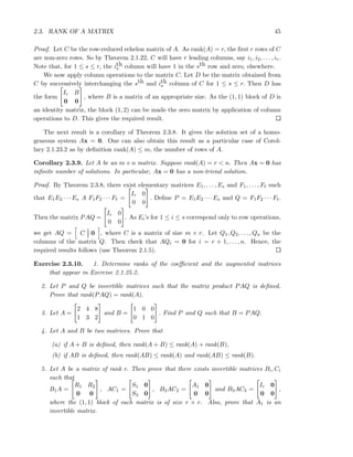
6. Let A be an m × n matrix of rank r. Then prove that A can be written as A = BC,
where both B and C have rank r and B is of size m × r and C is of size r × n.
7. Let A and B be two matrices such that AB is defined and rank(A) = rank(AB).
Then prove that A = ABX for some matrix X. Similarly, if BA is defined and
rank (A) = rank (BA), then A = Y BA for some matrix Y. [Hint: Choose invertible
matrices P, Q satisfying PAQ =
A1 0
0 0
, P(AB) = (PAQ)(Q−1
B) =
A2 A3
0 0
. Now find
R an invertible matrix with P(AB)R =
C 0
0 0
. Define X = R
C−1
A1 0
0 0
Q−1
.]
8. Suppose the matrices B and C are invertible and the involved partitioned products
are defined, then prove that
A B
C 0
−1
=
0 C−1
B−1 −B−1AC−1 .
9. Suppose A−1 = B with A =
A11 A12
A21 A22
and B =
B11 B12
B21 B22
. Also, assume that
A11 is invertible and define P = A22 − A21A−1
11 A12. Then prove that
(a) A is row-equivalent to the matrix
A11 A12
0 A22 − A21A−1
11 A12
,
(b) P is invertible and B =
A−1
11 + (A−1
11 A12)P−1(A21A−1
11 ) −(A−1
11 A12)P−1
−P−1(A21A−1
11 ) P−1 .
We end this section by giving another equivalent condition for a square matrix to be
invertible. To do so, we need the following definition.
Definition 2.3.11. A n × n matrix A is said to be of full rank if rank(A) = n.
Theorem 2.3.12. Let A be a square matrix of order n. Then the following statements are
equivalent.
1. A is invertible.
2. A has full rank.
3. The row-reduced form of A is In.
Proof. 1 =⇒ 2
Let if possible rank(A) = r < n. Then there exists an invertible matrix P (a product
of elementary matrices) such that PA =
B1 B2
0 0
, where B1 is an r × r matrix. Since A
is invertible, let A−1 =
C1
C2
, where C1 is an r × n matrix. Then
P = PIn = P(AA−1
) = (PA)A−1
=
B1 B2
0 0
C1
C2
=
B1C1 + B2C2
0
.](https://image.slidesharecdn.com/booklinear-160914134339/85/Book-linear-46-320.jpg)
![2.4. EXISTENCE OF SOLUTION OF AX = B 47
Thus, P has n − r rows consisting of only zeros. Hence, P cannot be invertible. A
contradiction. Thus, A is of full rank.
2 =⇒ 3
Suppose A is of full rank. This implies, the row-reduced echelon form of A has all
non-zero rows. But A has as many columns as rows and therefore, the last row of the
row-reduced echelon form of A is [0, 0, . . . , 0, 1]. Hence, the row-reduced echelon form of A
is In.
3 =⇒ 1
Using Theorem 2.2.5.3, the required result follows.
2.4 Existence of Solution of Ax = b
In Section 2.2, we studied the system of linear equations in which the matrix A was a square
matrix. We will now use the rank of a matrix to study the system of linear equations even
when A is not a square matrix. Before proceeding with our main result, we give an example
for motivation and observations. Based on these observations, we will arrive at a better
understanding, related to the existence and uniqueness results for the linear system Ax = b.
Consider a linear system Ax = b. Suppose the application of the Gauss-Jordan method
has reduced the augmented matrix [A b] to
[C d] =
1 0 2 −1 0 0 2 8
0 1 1 3 0 0 5 1
0 0 0 0 1 0 −1 2
0 0 0 0 0 1 1 4
0 0 0 0 0 0 0 0
0 0 0 0 0 0 0 0
.
Then to get the solution set, we observe the following.
Observations:
1. The number of non-zero rows in C is 4. This number is also equal to the number of
non-zero rows in [C d]. So, there are 4 leading columns/basic variables.
2. The leading terms appear in columns 1, 2, 5 and 6. Thus, the respective variables
x1, x2, x5 and x6 are the basic variables.
3. The remaining variables, x3, x4 and x7 are free variables.
Hence, the solution set is given by
x1
x2
x3
x4
x5
x6
x7
=
8 − 2x3 + x4 − 2x7
1 − x3 − 3x4 − 5x7
x3
x4
2 + x7
4 − x7
x7
=
8
1
0
0
2
4
0
+ x3
−2
−1
1
0
0
0
0
+ x4
1
−3
0
1
0
0
0
+ x7
−2
−5
0
0
1
−1
1
,](https://image.slidesharecdn.com/booklinear-160914134339/85/Book-linear-47-320.jpg)
![48 CHAPTER 2. SYSTEM OF LINEAR EQUATIONS
where x3, x4 and x7 are arbitrary.
Let x0 =
8
1
0
0
2
4
0
, u1 =
−2
−1
1
0
0
0
0
, u2 =
1
−3
0
1
0
0
0
and u3 =
−2
−5
0
0
1
−1
1
.
Then it can easily be verified that Cx0 = d, and for 1 ≤ i ≤ 3, Cui = 0. Hence, it follows
that Ax0 = d, and for 1 ≤ i ≤ 3, Aui = 0.
A similar idea is used in the proof of the next theorem and is omitted. The proof
appears on page 87 as Theorem 3.3.26.
Theorem 2.4.1 (Existence/Non-Existence Result). Consider a linear system Ax = b,
where A is an m × n matrix, and x, b are vectors of orders n × 1, and m × 1, respectively.
Suppose rank (A) = r and rank([A b]) = ra. Then exactly one of the following statement
holds:
1. If r < ra, the linear system has no solution.
2. if ra = r, then the linear system is consistent. Furthermore,
(a) if r = n then the solution set contains a unique vector x0 satisfying Ax0 = b.
(b) if r < n then the solution set has the form
{x0 + k1u1 + k2u2 + · · · + kn−run−r : ki ∈ R, 1 ≤ i ≤ n − r},
where Ax0 = b and Aui = 0 for 1 ≤ i ≤ n − r.
Remark 2.4.2. Let A be an m × n matrix. Then Theorem 2.4.1 implies that
1. the linear system Ax = b is consistent if and only if rank(A) = rank([A b]).
2. the vectors ui, for 1 ≤ i ≤ n − r, correspond to each of the free variables.
Exercise 2.4.3. In the introduction, we gave 3 figures (see Figure 2) to show the cases
that arise in the Euclidean plane (2 equations in 2 unknowns). It is well known that in the
case of Euclidean space (3 equations in 3 unknowns), there
1. is a figure to indicate the system has a unique solution.
2. are 4 distinct figures to indicate the system has no solution.
3. are 3 distinct figures to indicate the system has infinite number of solutions.
Determine all the figures.](https://image.slidesharecdn.com/booklinear-160914134339/85/Book-linear-48-320.jpg)
![2.5. DETERMINANT 49
2.5 Determinant
In this section, we associate a number with each square matrix. To do so, we start with the
following notation. Let A be an n×n matrix. Then for each positive integers αi’s 1 ≤ i ≤ k
and βj’s for 1 ≤ j ≤ ℓ, we write A(α1, . . . , αk β1, . . . , βℓ) to mean that submatrix of A,
that is obtained by deleting the rows corresponding to αi’s and the columns corresponding
to βj’s of A.
Example 2.5.1. Let A =
1 2 3
1 3 2
2 4 7
. Then A(1|2) =
1 2
2 7
, A(1|3) =
1 3
2 4
and
A(1, 2|1, 3) = [4].
With the notations as above, we have the following inductive definition of determinant
of a matrix. This definition is commonly known as the expansion of the determinant along
the first row. The students with a knowledge of symmetric groups/permutations can find
the definition of the determinant in Appendix 7.1.15. It is also proved in Appendix that
the definition given below does correspond to the expansion of determinant along the first
row.
Definition 2.5.2 (Determinant of a Square Matrix). Let A be a square matrix of order n.
The determinant of A, denoted det(A) (or |A|) is defined by
det(A) =
a, if A = [a] (n = 1),
n
j=1
(−1)1+ja1j det A(1|j) , otherwise.
Example 2.5.3. 1. Let A = [−2]. Then det(A) = |A| = −2.
2. Let A =
a b
c d
. Then, det(A) = |A| = a A(1|1) − b A(1|2) = ad − bc. For
example, if A =
1 2
3 5
then det(A) =
1 2
3 5
= 1 · 5 − 2 · 3 = −1.
3. Let A =
a11 a12 a13
a21 a22 a23
a31 a32 a33
. Then,
det(A) = |A| = a11 det(A(1|1)) − a12 det(A(1|2)) + a13 det(A(1|3))
= a11
a22 a23
a32 a33
− a12
a21 a23
a31 a33
+ a13
a21 a22
a31 a32
= a11(a22a33 − a23a32) − a12(a21a33 − a31a23)
+a13(a21a32 − a31a22) (2.5.1)
Let A =
1 2 3
2 3 1
1 2 2
. Then |A| = 1·
3 1
2 2
−2·
2 1
1 2
+3·
2 3
1 2
= 4−2(3)+3(1) = 1.](https://image.slidesharecdn.com/booklinear-160914134339/85/Book-linear-49-320.jpg)
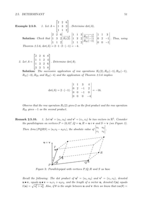
![2.5. DETERMINANT 53
Definition 2.5.13 (Adjoint of a Matrix). Let A be an n × n matrix. The matrix B = [bij]
with bij = Cji, for 1 ≤ i, j ≤ n is called the Adjoint of A, denoted Adj(A).
Example 2.5.14. Let A =
1 2 3
2 3 1
1 2 2
. Then Adj(A) =
4 2 −7
−3 −1 5
1 0 −1
as
C11 = (−1)1+1
A11 = 4, C21 = (−1)2+1
A21 = 2, . . . , C33 = (−1)3+3
A33 = −1.
Theorem 2.5.15. Let A be an n × n matrix. Then
1. for 1 ≤ i ≤ n,
n
j=1
aij Cij =
n
j=1
aij(−1)i+j Aij = det(A),
2. for i = ℓ,
n
j=1
aij Cℓj =
n
j=1
aij(−1)ℓ+j Aℓj = 0, and
3. A(Adj(A)) = det(A)In. Thus,
whenever det(A) = 0 one has A−1
=
1
det(A)
Adj(A). (2.5.2)
Proof. Part 1: It directly follows from Remark 2.5.8 and the definition of the cofactor.
Part 2: Fix positive integers i, ℓ with 1 ≤ i = ℓ ≤ n. And let B = [bij] be a square
matrix whose ℓth row equals the ith row of A and the remaining rows of B are the same
as that of A.
Then by construction, the ith and ℓth rows of B are equal. Thus, by Theorem 2.5.6.5,
det(B) = 0. As A(ℓ|j) = B(ℓ|j) for 1 ≤ j ≤ n, using Remark 2.5.8, we have
0 = det(B) =
n
j=1
(−1)ℓ+j
bℓj det B(ℓ|j) =
n
j=1
(−1)ℓ+j
aij det B(ℓ|j)
=
n
j=1
(−1)ℓ+j
aij det A(ℓ|j) =
n
j=1
aijCℓj. (2.5.3)
This completes the proof of Part 2.
Part 3:, Using Equation (2.5.3) and Remark 2.5.8, observe that
A Adj(A)
ij
=
n
k=1
aik Adj(A) kj
=
n
k=1
aikCjk =
0, if i = j,
det(A), if i = j.
Thus, A(Adj(A)) = det(A)In. Therefore, if det(A) = 0 then A 1
det(A)Adj(A) = In.
Hence, by Theorem 2.2.6,
A−1
=
1
det(A)
Adj(A).](https://image.slidesharecdn.com/booklinear-160914134339/85/Book-linear-53-320.jpg)
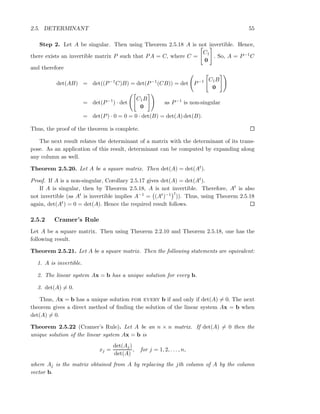
![56 CHAPTER 2. SYSTEM OF LINEAR EQUATIONS
Proof. Since det(A) = 0, A is invertible and hence the row-reduced echelon form of A is
I. Thus, for some invertible matrix P,
RREF[A|b] = P[A|b] = [PA|Pb] = [I|d],
where d = Ab. Hence, the system Ax = b has the unique solution xj = dj, for 1 ≤ j ≤ n.
Also,
[e1, e2, . . . , en] = I = PA = [PA[:, 1], PA[:, 2], . . . , PA[:, n]].
Thus,
PAj = P[A[:, 1], . . . , A[:, j − 1], b, A[:, j + 1], . . . , A[:, n]]
= [PA[:, 1], . . . , PA[:, j − 1], Pb, PA[:, j + 1], . . . , PA[:, n]]
= [e1, . . . , ej−1, d, ej+1, . . . , en]
and hence det(PAj) = dj, for 1 ≤ j ≤ n. Therefore,
det(Aj)
det(A)
=
det(P) det(Aj)
det(P) det(A)
=
det(PAj)
det(PA)
=
dj
1
= dj.
Hence, xj =
det(Aj )
det(A) and the required result follows.
In Theorem 2.5.22 A1 =
b1 a12 · · · a1n
b2 a22 · · · a2n
...
...
...
...
bn an2 · · · ann
, A2 =
a11 b1 a13 · · · a1n
a21 b2 a23 · · · a2n
...
...
...
...
...
an1 bn an3 · · · ann
and so
on till An =
a11 · · · a1n−1 b1
a12 · · · a2n−1 b2
...
...
...
...
a1n · · · ann−1 bn
.
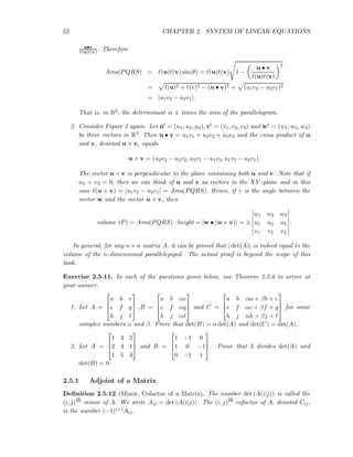
Example 2.5.23. Solve Ax = b using Cramer’s rule, where A =
1 2 3
2 3 1
1 2 2
and b =
1
1
1
.
Solution: Check that det(A) = 1 and xt = (−1, 1, 0) as
x1 =
1 2 3
1 3 1
1 2 2
= −1, x2 =
1 1 3
2 1 1
1 1 2
= 1, and x3 =
1 2 1
2 3 1
1 2 1
= 0.
2.6 Miscellaneous Exercises
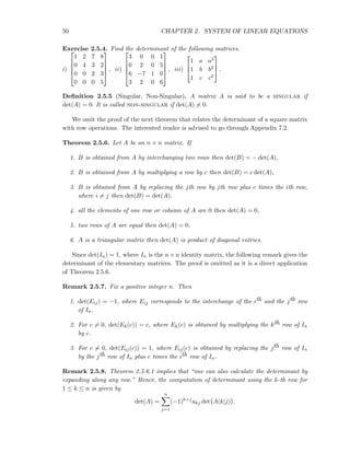
Exercise 2.6.1. 1. Show that a triangular matrix A is invertible if and only if each
diagonal entry of A is non-zero.
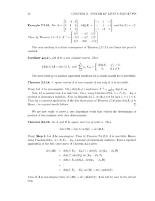
2. Let A be an orthogonal matrix. Prove that det A = ±1.](https://image.slidesharecdn.com/booklinear-160914134339/85/Book-linear-56-320.jpg)
![2.6. MISCELLANEOUS EXERCISES 57
3. Prove that every 2 × 2 matrix A satisfying tr(A) = 0 and det(A) = 0 is a nilpotent
matrix.
4. Let A and B be two non-singular matrices. Are the matrices A + B and A − B
non-singular? Justify your answer.
5. Let A be an n × n matrix. Prove that the following statements are equivalent:
(a) A is not invertible.
(b) rank(A) = n.
(c) det(A) = 0.
(d) A is not row-equivalent to In.
(e) The homogeneous system Ax = 0 has a non-trivial solution.
(f) The system Ax = b is either inconsistent or it is consistent and in this case it
has an infinite number of solutions.
(g) A is not a product of elementary matrices.
6. For what value(s) of λ does the following systems have non-trivial solutions? Also,
for each value of λ, determine a non-trivial solution.
(a) (λ − 2)x + y = 0, x + (λ + 2)y = 0.
(b) λx + 3y = 0, (λ + 6)y = 0.
7. Let x1, x2, . . . , xn be fixed reals numbers and define A = [aij]n×n with aij = xj−1
i .
Prove that det(A) =
1≤i<j≤n
(xj − xi). This matrix is usually called the Van-der
monde matrix.
8. Let A = [aij]n×n with aij = max{i, j}. Prove that det A = (−1)n−1n.
9. Let A = [aij]n×n with aij = 1
i+j−1. Using induction, prove that A is invertible. This
matrix is commonly known as the Hilbert matrix.
10. Solve the following system of equations by Cramer’s rule.
i) x + y + z − w = 1, x + y − z + w = 2, 2x + y + z − w = 7, x + y + z + w = 3.
ii) x − y + z − w = 1, x + y − z + w = 2, 2x + y − z − w = 7, x − y − z + w = 3.
11. Suppose A = [aij] and B = [bij] are two n × n matrices with bij = pi−jaij for
1 ≤ i, j ≤ n for some non-zero p ∈ R. Then compute det(B) in terms of det(A).
12. The position of an element aij of a determinant is called even or odd according as
i + j is even or odd. Show that
(a) If all the entries in odd positions are multiplied with −1 then the value of the
determinant doesn’t change.
(b) If all entries in even positions are multiplied with −1 then the determinant](https://image.slidesharecdn.com/booklinear-160914134339/85/Book-linear-57-320.jpg)
![58 CHAPTER 2. SYSTEM OF LINEAR EQUATIONS
i. does not change if the matrix is of even order.
ii. is multiplied by −1 if the matrix is of odd order.
13. Let A be a Hermitian (A∗ = At) matrix. Prove that det A is a real number.
14. Let A be an n × n matrix. Then A is invertible if and only if Adj(A) is invertible.
15. Let A and B be invertible matrices. Prove that Adj(AB) = Adj(B)Adj(A).
16. Let P =
A B
C D
be a rectangular matrix with A a square matrix of order n and
|A| = 0. Then show that rank (P) = n if and only if D = CA−1B.
2.7 Summary
In this chapter, we started with a system of linear equations Ax = b and related it to the
augmented matrix [A |b]. We applied row operations to [A |b] to get its row echelon form
and the row-reduced echelon forms. Depending on the row echelon matrix, say [C |d], thus
obtained, we had the following result:
1. If [C |d] has a row of the form [0 |1] then the linear system Ax = b has not solution.
2. Suppose [C |d] does not have any row of the form [0 |1] then the linear system Ax = b
has at least one solution.
(a) If the number of leading terms equals the number of unknowns then the system
Ax = b has a unique solution.
(b) If the number of leading terms is less than the number of unknowns then the
system Ax = b has an infinite number of solutions.
The following conditions are equivalent for an n × n matrix A.
1. A is invertible.
2. The homogeneous system Ax = 0 has only the trivial solution.
3. The row reduced echelon form of A is I.
4. A is a product of elementary matrices.
5. The system Ax = b has a unique solution for every b.
6. The system Ax = b has a solution for every b.
7. rank(A) = n.
8. det(A) = 0.
Suppose the matrix A in the linear system Ax = b is of size m × n. Then exactly one
of the following statement holds:](https://image.slidesharecdn.com/booklinear-160914134339/85/Book-linear-58-320.jpg)
![2.7. SUMMARY 59
1. if rank(A) < rank([A |b]), then the system Ax = b has no solution.
2. if rank(A) = rank([A |b]), then the system Ax = b is consistent. Furthermore,
(a) if rank(A) = n then the system Ax = b has a unique solution.
(b) if rank(A) < n then the system Ax = b has an infinite number of solutions.
We also dealt with the following type of problems:
1. Solving the linear system Ax = b. In the next chapter, we will see that this leads us
to the question “is the vector b a linear combination of the columns of A”?
2. Solving the linear system Ax = 0. In the next chapter, we will see that this leads us
to the question “are the columns of A linearly independent/dependent”?
(a) If Ax = 0 has a unique solution, the trivial solution, then the columns of A are
linear independent.
(b) If Ax = 0 has an infinite number of solutions then the columns of A are linearly
dependent.
3. Let bt = [b1, b2, . . . , bm]. Find conditions of the bi’s such that the linear system
Ax = b always has a solution. Observe that for different choices of x the vector Ax
gives rise to vectors that are linear combination of the columns of A. This idea will
be used in the next chapter, to get the geometrical representation of the linear span
of the columns of A.](https://image.slidesharecdn.com/booklinear-160914134339/85/Book-linear-59-320.jpg)

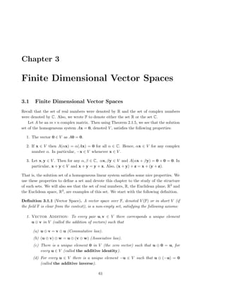
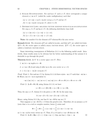
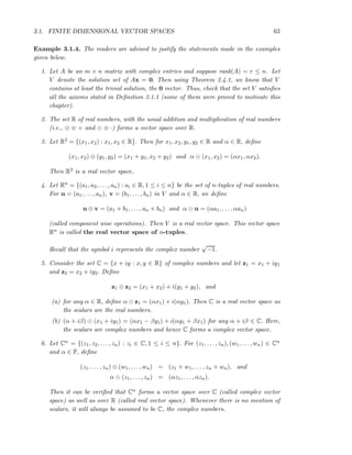
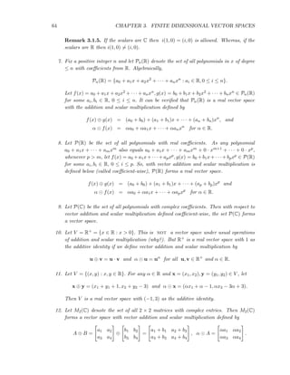
![3.1. FINITE DIMENSIONAL VECTOR SPACES 65
13. Fix positive integers m and n and let Mm×n(C) denote the set of all m × n matrices
with complex entries. Then Mm×n(C) is a vector space with vector addition and
scalar multiplication defined by
A ⊕ B = [aij] ⊕ [bij] = [aij + bij], α ⊙ A = α ⊙ [aij] = [αaij].
In case m = n, the vector space Mm×n(C) will be denoted by Mn(C).
14. Let C([−1, 1]) be the set of all real valued continuous functions on the interval [−1, 1].
Then C([−1, 1]) forms a real vector space if for all x ∈ [−1, 1], we define
(f ⊕ g)(x) = f(x) + g(x) for all f, g ∈ C([−1, 1]) and
(α ⊙ f)(x) = αf(x) for all α ∈ R and f ∈ C([−1, 1]).
15. Let V and W be vector spaces over F, with operations (+, •) and (⊕, ⊙), respectively.
Let V × W = {(v, w) : v ∈ V, w ∈ W}. Then V × W forms a vector space over F, if
for every (v1, w1), (v2, w2) ∈ V × W and α ∈ R, we define
(v1, w1) ⊕′
(v2, w2) = (v1 + v2, w1 ⊕ w2), and
α ◦ (v1, w1) = (α • v1, α ⊙ w1).
v1 + v2 and w1 ⊕ w2 on the right hand side mean vector addition in V and W,
respectively. Similarly, α • v1 and α ⊙ w1 correspond to scalar multiplication in V
and W, respectively.
From now on, we will use ‘u + v’ for ‘u ⊕ v’ and ‘α · u or αu’ for ‘α ⊙ u’.
Exercise 3.1.6. 1. Verify all the axioms are satisfied in all the examples of vector
spaces considered in Example 3.1.4.
2. Prove that the set Mm×n(R) for fixed positive integers m and n forms a real vector
space with usual operations of matrix addition and scalar multiplication.
3. Let V = {(x, y) : x, y ∈ R2}. For x = (x1, x2), y = (y1, y2) ∈ V , define
x + y = (x1 + y1, x2 + y2) and αx = (αx1, 0)
for all α ∈ R. Is V a vector space? Give reasons for your answer.
4. Let a, b ∈ R with a < b. Then prove that C([a, b]), the set of all complex valued
continuous functions on [a, b] forms a vector space if for all x ∈ [a, b], we define
(f ⊕ g)(x) = f(x) + g(x) for all f, g ∈ C([a, b]) and
(α ⊙ f)(x) = αf(x) for all α ∈ R and f ∈ C([a, b]).
5. Prove that C(R), the set of all real valued continuous functions on R forms a vector
space if for all x ∈ R, we define
(f ⊕ g)(x) = f(x) + g(x) for all f, g ∈ C(R) and
(α ⊙ f)(x) = αf(x) for all α ∈ R and f ∈ C(R).](https://image.slidesharecdn.com/booklinear-160914134339/85/Book-linear-65-320.jpg)
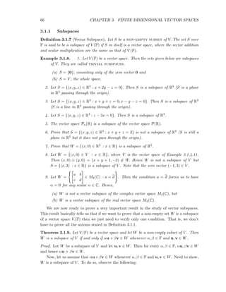
![3.1. FINITE DIMENSIONAL VECTOR SPACES 67
1. Taking α = 1 and β = 1, we see that u + v ∈ W for every u, v ∈ W.
2. Taking α = 0 and β = 0, we see that 0 ∈ W.
3. Taking β = 0, we see that αu ∈ W for every α ∈ F and u ∈ W and hence using
Theorem 3.1.3.3, −u = (−1)u ∈ W as well.
4. The commutative and associative laws of vector addition hold as they hold in V .
5. The axioms related with scalar multiplication and the distributive laws also hold as
they hold in V .
Thus, we have the required result.
Exercise 3.1.10. 1. Determine all the subspaces of R, R2 and R3.
2. Prove that a line in R2 is a subspace if and only if it passes through (0, 0) ∈ R2.
3. Let V = {(a, b) : a, b ∈ R}. Is V a vector space over R if (a, b) ⊕ (c, d) = (a + c, 0)
and α ⊙ (a, b) = (αa, 0)? Give reasons for your answer.
4. Let V = R. Define x ⊕ y = x − y and α ⊙ x = −αx. Which vector space axioms are
not satisfied here?
5. Which of the following are correct statements (why!)?
(a) S = {(x, y, z) ∈ R3 : z = x2} is a subspace of R3.
(b) S = {αx : α ∈ F} forms a vector subspace of V (F) for each fixed x ∈ V .
(c) S = {α(1, 1, 1) + β(1, −1, 0) : α, β ∈ R} is a vector subspace of R3.
(d) All the sets given below are subspaces of C([−1, 1]) (see Example 3.1.4.14).
i. W = {f ∈ C([−1, 1]) : f(1/2) = 0}.
ii. W = {f ∈ C([−1, 1]) : f(0) = 0, f(1/2) = 0}.
iii. W = {f ∈ C([−1, 1]) : f(−1/2) = 0, f(1/2) = 0}.
iv. W = {f ∈ C([−1, 1]) : f′(1
4 )exists }.
(e) All the sets given below are subspaces of P(R)?
i. W = {f(x) ∈ P(R) : deg(f(x)) = 3}.
ii. W = {f(x) ∈ P(R) : deg(f(x)) = 0}.
iii. W = {f(x) ∈ P(R) : f(1) = 0}.
iv. W = {f(x) ∈ P(R) : f(0) = 0, f(1) = 0}.
(f) Let A =
1 2 1
2 1 1
and b =
1
−1
. Then {x : Ax = b} is a subspace of R3.
(g) Let A =
1 2 1
2 1 1
. Then {x : Ax = 0} is a subspace of R3.
6. Which of the following are subspaces of Rn(R)?](https://image.slidesharecdn.com/booklinear-160914134339/85/Book-linear-67-320.jpg)
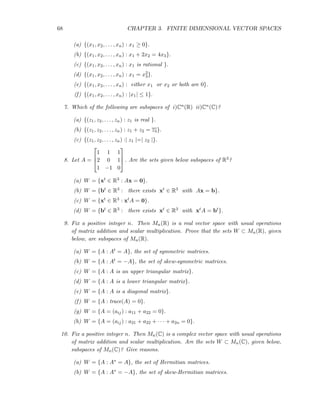
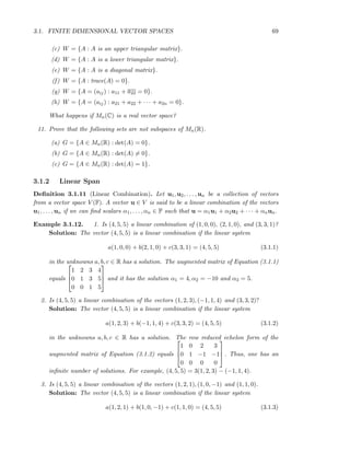
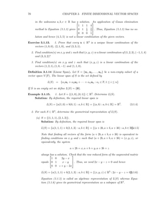
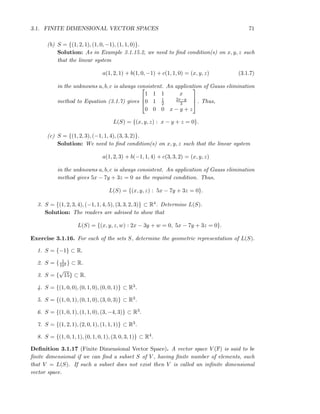
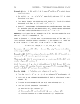
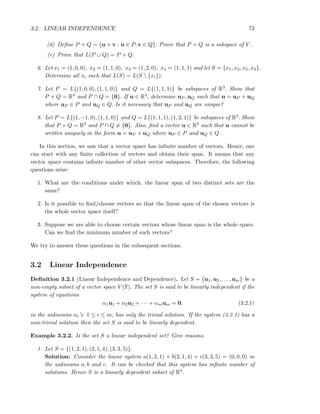
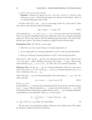
![3.2. LINEAR INDEPENDENCE 75
Corollary 3.2.5. Let S = {u1, . . . , un} be a subset of a vector space V (F). If S is linearly
1. dependent then there exists a k, 2 ≤ k ≤ n with L(u1, . . . , uk) = L(u1, . . . , uk−1).
2. independent and there is a vector v ∈ V with v ∈ L(S) then {u1, . . . , un, v} is also
a linearly independent subset of V.
Exercise 3.2.6. 1. Consider the vector space R2. Let u1 = (1, 0). Find all choices for
the vector u2 such that {u1, u2} is linearly independent subset of R2. Does there exist
vectors u2 and u3 such that {u1, u2, u3} is linearly independent subset of R2?
2. Let S = {(1, 1, 1, 1), (1, −1, 1, 2), (1, 1, −1, 1)} ⊂ R4. Does (1, 1, 2, 1) ∈ L(S)? Further-
more, determine conditions on x, y, z and u such that (x, y, z, u) ∈ L(S).
3. Show that S = {(1, 2, 3), (−2, 1, 1), (8, 6, 10)} ⊂ R3 is linearly dependent.
4. Show that S = {(1, 0, 0), (1, 1, 0), (1, 1, 1)} ⊂ R3 is linearly independent.
5. Prove that {u1, u2, . . . , un} is a linearly independent subset of V (F) if and only if
{u1, u1 + u2, . . . , u1 + · · · + un} is linearly independent subset of V (F).
6. Find 3 vectors u, v and w in R4 such that {u, v, w} is linearly dependent whereas
{u, v}, {u, w} and {v, w} are linearly independent.
7. What is the maximum number of linearly independent vectors in R3?
8. Show that any set of k vectors in R3 is linearly dependent if k ≥ 4.
9. Is {(1, 0), (i, 0)} a linearly independent subset of C2 (R)?
10. Suppose V is a collection of vectors such that V (C) as well as V (R) are vector spaces.
Prove that the set {u1, . . . , uk, iu1, . . . , iuk} is a linearly independent subset of V (R)
if and only if {u1, . . . , uk} is a linear independent subset of V (C).
11. Let M be a subspace of V and let u, v ∈ V . Define K = L(M, u) and H = L(M, v).
If v ∈ K and v ∈ M prove that u ∈ H.
12. Let A ∈ Mn(R) and let x and y be two non-zero vectors such that Ax = 3x and
Ay = 2y. Prove that x and y are linearly independent.
13. Let A =
2 1 3
4 −1 3
3 −2 5
. Determine non-zero vectors x, y and z such that Ax = 6x,
Ay = 2y and Az = −2z. Use the vectors x, y and z obtained here to prove the
following.
(a) A2v = 4v, where v = cy + dz for any real numbers c and d.
(b) The set {x, y, z} is linearly independent.
(c) Let P = [x, y, z] be a 3 × 3 matrix. Then P is invertible.](https://image.slidesharecdn.com/booklinear-160914134339/85/Book-linear-75-320.jpg)
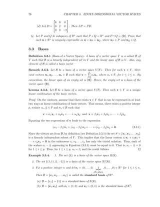
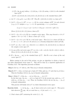
![3.3. BASES 81
3. Consider the vector space C([−π, π]). For each integer n, define en(x) = sin(nx).
Prove that {en : n = 1, 2, . . .} is a linearly independent set.
[Hint: For any positive integer ℓ, consider the set {ek1 , . . . , ekℓ
} and the linear system
α1 sin(k1x) + α2 sin(k2x) + · · · + αℓ sin(kℓx) = 0 for all x ∈ [−π, π]
in the unknowns α1, . . . , αn. Now for suitable values of m, consider the integral
π
−π
sin(mx) (α1 sin(k1x) + α2 sin(k2x) + · · · + αℓ sin(kℓx)) dx
to get the required result.]
4. Determine a basis and dimension of W = {(x, y, z, w) ∈ R4 : x + y − z + w = 0}.
5. Let W1 be a subspace of a vector space V . If dim(V ) = n and dim(W1) = k with
k ≥ 1 then prove that there exists a subspace W2 of V such that W1 ∩ W2 = {0},
W1 + W2 = V and dim(W2) = n − k. Also, prove that for each v ∈ V there exist
unique vectors w1 ∈ W1 and w2 ∈ W2 such that v = w1 + w2. The subspace W2 is
called the complementary subspace of W1 in V.
6. Is the set, W = {p(x) ∈ P4(R) : p(−1) = p(1) = 0} a subspace of P4(R)? If yes,
find its dimension.
3.3.2 Application to the study of Cn
In this subsection, we will study results that are intrinsic to the understanding of linear
algebra, especially results associated with matrices. We start with a few exercises that
should have appeared in previous sections of this chapter.
Exercise 3.3.14. 1. Let V = {A ∈ M2(C) : tr(A) = 0}, where tr(A) stands for the
trace of the matrix A. Show that V is a real vector space and find its basis. Is
W =
a b
c −a
: c = −b a subspace of V ?
2. In each of the questions given below, determine whether the given set is a vector space
or not? If it is a vector space, find the dimension and a basis.
(a) sln(R) = {A ∈ Mn(R) : tr(A) = 0}.
(b) Sn(R) = {A ∈ Mn(R) : A = At}.
(c) An(R) = {A ∈ Mn(R) : A + At = 0}.
(d) sln(C) = {A ∈ Mn(C) : tr(A) = 0}.
(e) Sn(C) = {A ∈ Mn(C) : A = A∗}.
(f) An(C) = {A ∈ Mn(C) : A + A∗ = 0}.
3. Does there exist an A ∈ M2(C) satisfying A2 = 0 but A3 = 0.
4. Prove that there does not exist an A ∈ Mn(C) satisfying An = 0 but An+1 = 0. That
is, if A is an n × n nilpotent matrix then the order of nilpotency ≤ n.](https://image.slidesharecdn.com/booklinear-160914134339/85/Book-linear-81-320.jpg)
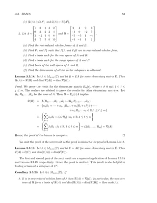
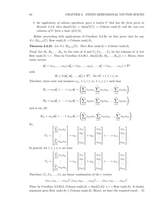
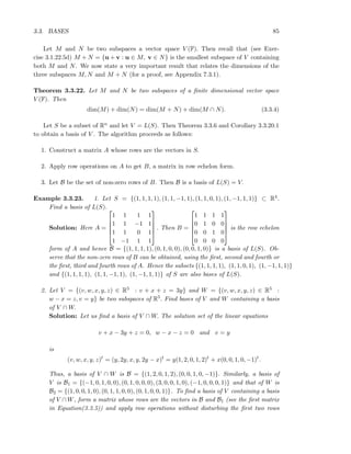
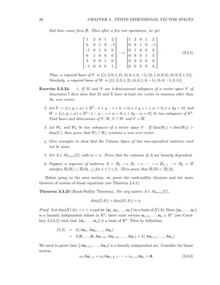
![3.3. BASES 87
in the unknowns α1, . . . , αn−r. This linear system is equivalent to
A(α1ur+1 + α2ur+2 + · · · + αn−run) = 0.
Hence, by definition of N(A), α1ur+1 + · · · + αn−run ∈ N(A) = L(u1, . . . , ur). Therefore,
there exists scalars βi, 1 ≤ i ≤ r such that
α1ur+1 + α2ur+2 + · · · + αn−run = β1u1 + β2u2 + · · · + βrur.
Or equivalently,
β1u1 + · · · + βrur − α1ur+1 − · · · − αn−run = 0. (3.3.7)
As {u1, . . . , un} is a linearly independent set, the only solution of Equation (3.3.7) is
αi = 0 for 1 ≤ i ≤ n − r and βj = 0 for 1 ≤ j ≤ r.
In other words, we have shown that the only solution of Equation (3.3.6) is the trivial
solution (αi = 0 for all i, 1 ≤ i ≤ n − r). Hence, the set {Aur+1, . . . , Aun} is a linearly
independent and is a basis of C(A). Thus
dim(C(A)) + dim(N(A)) = (n − r) + r = n
and the proof of the theorem is complete.
Theorem 3.3.25 is part of what is known as the fundamental theorem of linear algebra
(see Theorem 5.2.15). As the final result in this direction, We now prove the main theorem
on linear systems stated on page 48 (see Theorem 2.4.1) whose proof was omitted.
Theorem 3.3.26. Consider a linear system Ax = b, where A is an m × n matrix, and
x, b are vectors of orders n × 1, and m × 1, respectively. Suppose rank (A) = r and
rank([A b]) = ra. Then exactly one of the following statement holds:
1. If r < ra, the linear system has no solution.
2. if ra = r, then the linear system is consistent. Furthermore,
(a) if r = n, then the solution set of the linear system has a unique n × 1 vector x0
satisfying Ax0 = b.
(b) if r < n, then the set of solutions of the linear system is an infinite set and has
the form
{x0 + k1u1 + k2u2 + · · · + kn−run−r : ki ∈ R, 1 ≤ i ≤ n − r},
where x0, u1, . . . , un−r are n × 1 vectors satisfying Ax0 = b and Aui = 0 for
1 ≤ i ≤ n − r.](https://image.slidesharecdn.com/booklinear-160914134339/85/Book-linear-87-320.jpg)
![88 CHAPTER 3. FINITE DIMENSIONAL VECTOR SPACES
Proof. Proof of Part 1. As r < ra, the (r + 1)-th row of the row-reduced echelon form of
[A b] has the form [0, 1]. Thus, by Theorem 1, the system Ax = b is inconsistent.
Proof of Part 2a and Part 2b. As r = ra, using Corollary 3.3.20, C(A) = C([A, b]).
Hence, the vector b ∈ C(A) and therefore there exist scalars c1, c2, . . . , cn such that b =
c1a1 +c2a2 +· · · cnan, where a1, a2, . . . , an are the columns of A. That is, we have a vector
xt
0 = [c1, c2, . . . , cn] that satisfies Ax = b.
If in addition r = n, then the system Ax = b has no free variables in its solution set
and thus we have a unique solution (see Theorem 2.1.22.2a).
Whereas the condition r < n implies that the system Ax = b has n−r free variables in
its solution set and thus we have an infinite number of solutions (see Theorem 2.1.22.2b).
To complete the proof of the theorem, we just need to show that the solution set in this
case has the form {x0 + k1u1 + k2u2 + · · · + kn−run−r : ki ∈ R, 1 ≤ i ≤ n − r}, where
Ax0 = b and Aui = 0 for 1 ≤ i ≤ n − r.
To get this, note that using the rank-nullity theorem (see Theorem 3.3.25) rank(A) = r
implies that dim(N(A)) = n − r. Let {u1, u2, . . . , un−r} be a basis of N(A). Then by
definition Aui = 0 for 1 ≤ i ≤ n − r and hence
A(x0 + k1u1 + k2u2 + · · · + kn−run−r) = Ax0 + k10 + · · · + kn−r0 = b.
Thus, the required result follows.
Example 3.3.27. Let A =
1 1 0 1 1 0 −1
0 0 1 2 3 0 −2
0 0 0 0 0 1 1
and V = {xt ∈ R7 : Ax = 0}. Find
a basis and dimension of V .
Solution: Observe that x1, x3 and x6 are the basic variables and the rest are the free
variables. Writing the basic variables in terms of free variables, we get
x1 = x7 − x2 − x4 − x5, x3 = 2x7 − 2x4 − 3x5 and x6 = −x7.
Hence,
x1
x2
x3
x4
x5
x6
x7
=
x7 − x2 − x4 − x5
x2
2x7 − 2x4 − 3x5
x4
x5
−x7
x7
= x2
−1
1
0
0
0
0
0
+ x4
−1
0
−2
1
0
0
0
+ x5
−1
0
−3
0
1
0
0
+ x7
1
0
2
0
0
−1
1
. (3.3.8)
Therefore, if we let ut
1 = −1, 1, 0, 0, 0, 0, 0 , ut
2 = −1, 0, −2, 1, 0, 0, 0 , ut
3 = −1, 0, −3, 0, 1, 0, 0
and ut
4 = 1, 0, 2, 0, 0, −1, 1 then S = {u1, u2, u3, u4} is the basis of V . The reasons are
as follows:](https://image.slidesharecdn.com/booklinear-160914134339/85/Book-linear-88-320.jpg)
![90 CHAPTER 3. FINITE DIMENSIONAL VECTOR SPACES
3.4 Ordered Bases
Let B = {u1, u2, . . . , un} be a basis of a vector space V . As B is a set, there is no ordering
of its elements. In this section, we want to associate an order among the vectors in any
basis of V as this helps in getting a better understanding about finite dimensional vector
spaces and its relationship with matrices.
Definition 3.4.1 (Ordered Basis). Let V be a vector space of dimension n. Then an
ordered basis for V is a basis {u1, u2, . . . , un} together with a one-to-one correspondence
between the sets {u1, u2, . . . , un} and {1, 2, 3, . . . , n}.
If the ordered basis has u1 as the first vector, u2 as the second vector and so on, then
we denote this by writing the ordered basis as (u1, u2, . . . , un).
Example 3.4.2. 1. Consider the vector space P2(R) with basis {1− x, 1+ x, x2}. Then
one can take either B1 = 1− x, 1+ x, x2 or B2 = 1+ x, 1− x, x2 as ordered bases.
Also for any element a0 + a1x + a2x2 ∈ P2(R), one has
a0 + a1x + a2x2
=
a0 − a1
2
(1 − x) +
a0 + a1
2
(1 + x) + a2x2
.
Thus, a0 + a1x + a2x2 in the ordered basis
(a) B1, has a0−a1
2 as the coefficient of the first element, a0+a1
2 as the coefficient of
the second element and a2 as the coefficient the third element of B1.
(b) B2, has a0+a1
2 as the coefficient of the first element, a0−a1
2 as the coefficient of
the second element and a2 as the coefficient the third element of B2.
2. Let V = {(x, y, z) : x+y = z} and let B = {(−1, 1, 0), (1, 0, 1)} be a basis of V . Then
check that (3, 4, 7) = 4(−1, 1, 0) + 7(1, 0, 1) ∈ V.
That is, as ordered bases (u1, u2, . . . , un), (u2, u3, . . . , un, u1) and (un, un−1, . . . , u2, u1)
are different even though they have the same set of vectors as elements. To proceed further,
we now define the notion of coordinates of a vector depending on the chosen ordered basis.
Definition 3.4.3 (Coordinates of a Vector). Let B = (v1, v2, . . . , vn) be an ordered basis
of a vector space V and let v ∈ V . Suppose
v = β1v1 + β2v2 + · · · + βnvn for some scalars β1, β2, . . . , βn.
Then the tuple (β1, β2, . . . , βn)t is called the coordinate of the vector v with respect to the
ordered basis B and is denoted by [v]B = (β1, . . . , βn)t, a column vector.
Example 3.4.4. 1. In Example 3.4.2.1, let p(x) = a0 + a1x + a2x2. Then
[p(x)]B1 =
a0−a1
2
a0+a1
2
a2
, [p(x)]B2 =
a0+a1
2
a0−a1
2
a2
and [p(x)]B3 =
a2
a0−a1
2
a0+a1
2
.](https://image.slidesharecdn.com/booklinear-160914134339/85/Book-linear-90-320.jpg)
![3.4. ORDERED BASES 91
2. In Example 3.4.2.2, (3, 4, 7) B
=
4
7
and (x, y, z) B
= (z − y, y, z) B
=
y
z
.
3. Let the ordered bases of R3 be B1 = (1, 0, 0), (0, 1, 0), (0, 0, 1) , B2 = (1, 0, 0), (1, 1, 0), (1, 1, 1)
and B3 = (1, 1, 1), (1, 1, 0), (1, 0, 0) . Then
(1, −1, 1) = 1 · (1, 0, 0) + (−1) · (0, 1, 0) + 1 · (0, 0, 1).
= 2 · (1, 0, 0) + (−2) · (1, 1, 0) + 1 · (1, 1, 1).
= 1 · (1, 1, 1) + (−2) · (1, 1, 0) + 2 · (1, 0, 0).
Therefore, if we write u = (1, −1, 1), then
[u]B1 = (1, −1, 1)t
, [u]B2 = (2, −2, 1)t
, [u]B3 = (1, −2, 2)t
.
In general, let V be an n-dimensional vector space with B1 = (u1, u2, . . . , un) and
B2 = (v1, v2, . . . , vn). Since B1 is a basis of V, there exist unique scalars aij, 1 ≤ i, j ≤ n,
such that
vi =
n
l=1
aliul, or equivalently, [vi]B1 = (a1i, a2i, . . . , ani)t
for 1 ≤ i ≤ n.
Suppose v ∈ V with [v]B2 = (α1, α2, . . . , αn)t. Then
v =
n
i=1
αivi =
n
i=1
αi
n
j=1
ajiuj
=
n
j=1
n
i=1
ajiαi uj.
Since B1 is a basis this representation of v in terms of ui’s is unique. So,
[v]B1 =
n
i=1
a1iαi,
n
i=1
a2iαi, . . . ,
n
i=1
aniαi
t
=
a11 · · · a1n
a21 · · · a2n
...
...
...
an1 · · · ann
α1
α2
...
αn
= A[v]B2 ,
where A = [v1]B1 , [v2]B1 , . . . , [vn]B1 . Hence, we have proved the following theorem.
Theorem 3.4.5. Let V be an n-dimensional vector space with bases B1 = (u1, u2, . . . , un)
and B2 = (v1, v2, . . . , vn). Define an n × n matrix A by A = [v1]B1 , [v2]B1 , . . . , [vn]B1 .
Then, A is an invertible matrix (see Exercise 3.3.14.7) and
[v]B1 = A[v]B2 for all v ∈ V.
Theorem 3.4.5 states that the coordinates of a vector with respect to different bases
are related via an invertible matrix A.
Example 3.4.6. Let B1 = (1, 0, 0), (1, 1, 0), (1, 1, 1) and B2 = (1, 1, 1), (1, −1, 1), (1, 1, 0)
be two bases of R3.](https://image.slidesharecdn.com/booklinear-160914134339/85/Book-linear-91-320.jpg)
![92 CHAPTER 3. FINITE DIMENSIONAL VECTOR SPACES
1. Then [(x, y, z)]B1 = (x − y, y − z, z)t and [(x, y, z)]B2 = (y−x
2 + z, x−y
2 , x − z)t.
2. Check that A = [(1, 1, 1)]B1 , [(1, −1, 1)]B1 , [(1, 1, 0)]B1 =
0 2 0
0 −2 1
1 1 0
as
[(1, 1, 1)]B1
= 0 · (1, 0, 0) + 0 · (1, 1, 0) + 1 · (1, 1, 1) = (0, 0, 1)t
,
[(1, −1, 1)]B1
= 2 · (1, 0, 0) + (−2) · (1, 1, 0) + 1 · (1, 1, 1) = (2, −2, 1)t
and
[(1, 1, 0)]B1
= 0 · (1, 0, 0) + 1 · (1, 1, 0) + 0 · (1, 1, 1) = (0, 1, 0)t
.
3. Thus, for any (x, y, z) ∈ R3,
[(x, y, z)]B1 =
x − y
y − z
z
=
0 2 0
0 −2 1
1 1 0
y−x
2 + z
x−y
2
x − z
= A [(x, y, z)]B2 .
4. Observe that the matrix A is invertible and hence [(x, y, z)]B2 = A−1 [(x, y, z)]B1 .
In the next chapter, we try to understand Theorem 3.4.5 again using the ideas of ‘linear
transformations/functions’.
Exercise 3.4.7. 1. Consider the vector space P3(R).
(a) Prove that B1 = (1−x, 1+x2, 1−x3, 3+x2 −x3) and B2 = (1, 1−x, 1+x2, 1−x3)
are bases of P3(R).
(b) Find the coordinates of u = 1 + x + x2 + x3 with respect to B1 and B2.
(c) Find the matrix A such that [u]B2 = A[u]B1 .
(d) Let v = a0 + a1x + a2x2 + a3x3. Then verify that
[v]B1 =
−a1
−a0 − a1 + 2a2 − a3
−a0 − a1 + a2 − 2a3
a0 + a1 − a2 + a3
=
0 1 0 0
−1 0 1 0
−1 0 0 1
1 0 0 0
a0 + a1 − a2 + a3
−a1
a2
−a3
= [v]B2 .
2. Let B = (2, 1, 0), (2, 1, 1), (2, 2, 1) be an ordered basis of R3. Determine the coordi-
nates of (1, 2, 1) and (4, −2, 2) with respect B.
3.5 Summary
In this chapter, we started with the definition of vector spaces over F, the set of scalars.
The set F was either R, the set of real numbers or C, the set of complex numbers.
It was important to note that given a non-empty set V of vectors with a set F of scalars,
we need to do the following:
1. first define vector addition and scalar multiplication and](https://image.slidesharecdn.com/booklinear-160914134339/85/Book-linear-92-320.jpg)
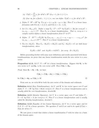
![4.1. DEFINITIONS AND BASIC PROPERTIES 97
Theorem 4.1.7. Let V and W be two vector spaces over F and let T : V −→W be a
linear transformation. If B = u1, . . . , un is an ordered basis of V then for each v ∈ V ,
the vector T(v) is a linear combination of T(u1), . . . , T(un) ∈ W. That is, we have full
information of T if we know T(u1), . . . , T(un) ∈ W, the image of basis vectors in W.
Proof. As B is a basis of V, for every v ∈ V, we can find c1, . . . , cn ∈ F such that v =
c1u1 + · · · + cnun, or equivalently [v]B = (α1, . . . , αn)t. Hence, by definition
T(v) = T(c1u1 + · · · + cnun) = c1T(u1) + · · · + cnT(un).
That is, we just need to know the vectors T(u1), T(u2), . . . , T(un) in W to get T(v) as
[v]B = (α1, . . . , αn)t is known in V . Hence, the required result follows.
Exercise 4.1.8. 1. Are the maps T : V −→W given below, linear transformations?
(a) Let V = R2 and W = R3 with T(x, y) = (x + y + 1, 2x − y, x + 3y).
(b) Let V = W = R2 with T(x, y) = (x − y, x2 − y2).
(c) Let V = W = R2 with T(x, y) = (x − y, |x|).
(d) Let V = R2 and W = R4 with T(x, y) = (x + y, x − y, 2x + y, 3x − 4y).
(e) Let V = W = R4 with T(x, y, z, w) = (z, x, w, y).
2. Which of the following maps T : M2(R)−→M2(R) are linear operators?
(a) T(A) = At (b) T(A) = I + A (c) T(A) = A2
(d) T(A) = BAB−1, where B is a fixed 2 × 2 matrix.
3. Prove that a map T : R −→ R is a linear transformation if and only if there exists a
unique c ∈ R such that T(x) = cx for every x ∈ R.
4. Let A ∈ Mn(C) and define TA : Cn−→Cn by TA(xt) = Ax for every xt ∈ Cn. Prove
that for any positive integer k, Tk
A(xt) = Akx.
5. Use matrices to give examples of linear operators T, S : R3−→R3 that satisfy:
(a) T = 0, T2 = 0, T3 = 0.
(b) T = 0, S = 0, S ◦ T = 0, T ◦ S = 0.
(c) S2 = T2, S = T.
(d) T2 = I, T = I.
6. Let T : Rn −→ Rn be a linear operator with T = 0 and T2 = 0. Prove that there
exists a vector x ∈ Rn such that the set {x, T(x)} is linearly independent.
7. Fix a positive integer p and let T : Rn −→ Rn be a linear operator with Tk = 0 for
1 ≤ k ≤ p and Tp+1 = 0. Then prove that there exists a vector x ∈ Rn such that the
set {x, T(x), . . . , Tp(x)} is linearly independent.](https://image.slidesharecdn.com/booklinear-160914134339/85/Book-linear-97-320.jpg)
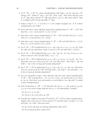
![4.2. MATRIX OF A LINEAR TRANSFORMATION 99
4.2 Matrix of a linear transformation
In the previous section, we learnt the definition of a linear transformation. We also saw
in Example 4.1.2.5 that for each A ∈ Mm×n(C), there exists a linear transformation TA :
Cn−→Cm given by TA(xt) = Ax for each xt ∈ Cn. In this section, we prove that every
linear transformation over finite dimensional vector spaces corresponds to a matrix. Before
proceeding further, we advise the reader to recall the results on ordered basis, studied in
Section 3.4.
Let V and W be finite dimensional vector spaces over F with dimensions n and m,
respectively. Also, let B1 = (v1, . . . , vn) and B2 = (w1, . . . , wm) be ordered bases of V
and W, respectively. If T : V −→W is a linear transformation then Theorem 4.1.7 implies
that T(v) ∈ W is a linear combination of the vectors T(v1), . . . , T(vn). So, let us find the
coordinate vectors [T(vj)]B2 for each j = 1, 2, . . . , n. Let us assume that
[T(v1)]B2
= (a11, . . . , am1)t
, [T(v2)]B2
= (a12, . . . , am2)t
, . . . , [T(vn)]B2
= (a1n, . . . , amn)t
.
Or equivalently,
T(vj) = a1jw1 + a2jw2 + · · · + amjwm =
m
i=1
aijwi for j = 1, 2, . . . , n. (4.2.1)
Therefore, for a fixed x ∈ V , if [x]B1 = (x1, x2, . . . , xn)t then
T(x) = T
n
j=1
xjvj
=
n
j=1
xjT(vj) =
n
j=1
xj
m
i=1
aijwi =
m
i=1
n
j=1
aijxj
wi.
(4.2.2)
Hence, using Equation (4.2.2), the coordinates of T(x) with respect to the basis B2 equals
[T(x)]B2 =
n
j=1
a1jxj
...
n
j=1
amjxj
=
a11 a12 · · · a1n
a21 a22 · · · a2n
...
...
...
...
am1 am2 · · · amn
x1
x2
...
xn
= A [x]B1 ,
where
A =
a11 a12 · · · a1n
a21 a22 · · · a2n
...
...
...
...
am1 am2 · · · amn
= [T(v1)]B2
, [T(v2)]B2
, . . . , [T(vn)]B2
. (4.2.3)
The above observations lead to the following theorem and the subsequent definition.
Theorem 4.2.1. Let V and W be finite dimensional vector spaces over F with dimensions
n and m, respectively. Let T : V −→W be a linear transformation. Also, let B1 and B2 be
ordered bases of V and W, respectively. Then there exists a matrix A ∈ Mm×n(F), denoted
A = T[B1, B2], with A = [T(v1)]B2
, [T(v2)]B2
, . . . , [T(vn)]B2
such that
[T(x)]B2 = A [x]B1 .](https://image.slidesharecdn.com/booklinear-160914134339/85/Book-linear-99-320.jpg)
![100 CHAPTER 4. LINEAR TRANSFORMATIONS
Definition 4.2.2 (Matrix of a Linear Transformation). Let V and W be finite dimensional
vector spaces over F with dimensions n and m, respectively. Let T : V −→W be a linear
transformation. Then the matrix T[B1, B2] is called the matrix of the linear transformation
with respect to the ordered bases B1 and B2.
Remark 4.2.3. Let B1 = (v1, . . . , vn) and B2 = (w1, . . . , wm) be ordered bases of V and
W, respectively. Also, let T : V −→ W be a linear transformation. Then writing T[B1, B2]
in place of the matrix A, Equation (4.2.1) can be rewritten as
T(vj) =
m
i=1
T[B1, B2]ijwi, for 1 ≤ j ≤ n. (4.2.4)
We now give a few examples to understand the above discussion and Theorem 4.2.1.
Q = (0, 1)
P = (1, 0)θ
θ
Q′ = (− sin θ, cos θ)
P′ = (cos θ, sin θ)
θ
α
P = (x, y)
P′ = (x′, y′)
Figure 4.1: Counter-clockwise Rotation by an angle θ
Example 4.2.4. 1. Let T : R2−→R2 be a function that counterclockwise rotates every
point in R2 by an angle θ, 0 ≤ θ < 2π. Then using Figure 4.1 it can be checked that
x′ = OP′ cos(α + θ) = OP cos α cos θ − sin α sin θ = x cos θ − y sin θ and similarly
y′ = x sin θ + y cos θ. Or equivalently, if B = (e1, e2) is the standard ordered basis of
R2, then using T(1, 0) = (cos θ, sin θ) and T(0, 1) = (− sin θ, cos θ), we get
T[B, B] = [T(1, 0)]B, [T(0, 1)]B =
cos θ − sin θ
sin θ cos θ
. (4.2.5)
2. Let B1 = (1, 0), (0, 1) and B2 = (1, 1), (1, −1) be two ordered bases of R2. Then
Compute T[B1, B1] and T[B2, B2] for the linear transformation T : R2−→R2 defined
by T(x, y) = (x + y, x − 2y).
Solution: Observe that for (x, y) ∈ R2, [(x, y)]B1 =
x
y
and [(x, y)]B2 =
x+y
2
x−y
2
.
Also, T(1, 0) = (1, 1), T(0, 1) = (1, −2), T(1, 1) = (2, −1) and T(1, −1) = (0, 3).
Thus, we have
T[B1, B1] = [T 1, 0) ]B1 , [T 0, 1) ]B1 = [(1, 1)]B1 , [(1, −2)]B1 =
1 1
1 −2
and
T[B2, B2] = [T 1, 1) ]B2 , [T 1, −1) ]B2 = [(2, −1)]B2 , [(0, 3)]B2 =
1
2
3
2
3
2 −3
2
.](https://image.slidesharecdn.com/booklinear-160914134339/85/Book-linear-100-320.jpg)
![4.2. MATRIX OF A LINEAR TRANSFORMATION 101
Hence, we see that
[T(x, y)]B1
= (x + y, x − 2y) B1
=
x + y
x − 2y
=
1 1
1 −2
x
y
and
[T(x, y)]B2
= (x + y, x − 2y) B2
=
2x−y
2
3y
2
=
1
2
3
2
3
2 −3
2
x+y
2
x−y
2
3. Let B1 = (1, 0, 0), (0, 1, 0), (0, 0, 1) and B2 = (1, 0), (0, 1) be ordered bases of R3
and R2, respectively. Define T : R3−→R2 by T(x, y, z) = (x + y − z, x + z). Then
T[B1, B2] = [(1, 0, 0)]B2 , [(0, 1, 0)]B2 , [(0, 0, 1)]B2 =
1 1 −1
1 0 1
.
Check that [T(x, y, z)]B2 = (x + y − z, x + z)t = T[B1, B2] [(x, y, z)]B1 .
4. Let B1 = (1, 0, 0), (0, 1, 0), (0, 0, 1) , B2 = (1, 0, 0), (1, 1, 0), (1, 1, 1) be two ordered
bases of R3. Define T : R3−→R3 by T(xt) = x for all xt ∈ R3. Then
[T(1, 0, 0)]B2
= 1 · (1, 0, 0) + 0 · (1, 1, 0) + 0 · (1, 1, 1) = (1, 0, 0)t
,
[T(0, 1, 0)]B2
= −1 · (1, 0, 0) + 1 · (1, 1, 0) + 0 · (1, 1, 1) = (−1, 1, 0)t
, and
[T(0, 0, 1)]B2
= 0 · (1, 0, 0) + (−1) · (1, 1, 0) + 1 · (1, 1, 1) = (0, −1, 1)t
.
Thus, check that
T[B1, B2] = [[T(1, 0, 0)]B2 , [T(0, 1, 0)]B2 , [T(0, 0, 1)]B2 ]
= [(1, 0, 0)t
, (−1, 1, 0)t
, (0, −1, 1)t
] =
1 −1 0
0 1 −1
0 0 1
,
T[B2, B1] = [[T(1, 0, 0)]B1 , [T(1, 1, 0)]B1 , [T(1, 1, 1)]B1 ] =
1 1 1
0 1 1
0 0 1
,
T[B1, B1] = I3 = T[B2, B2] and T[B2, B1]−1 = T[B1, B2].
Remark 4.2.5. 1. Let V and W be finite dimensional vector spaces over F with order
bases B1 = (v1, . . . , vn) and B2 of V and W, respectively. If T : V −→W is a linear
transformation then
(a) T[B1, B2] = [T(v1)]B2 , [T(v2)]B2 , . . . , [T(vn)]B2 .
(b) [T(x)]B2 = T[B1, B2] [x]B1 for all x ∈ V . That is, the coordinate vector of
T(x) ∈ W is obtained by multiplying the matrix of the linear transformation
with the coordinate vector of x ∈ V .
2. Let A ∈ Mm×n(R). Then A induces a linear transformation TA : Rn−→Rm defined
by TA(xt) = Ax for all xt ∈ Rn. Let B1 and B2 be the standard ordered bases of Rn
and Rm, respectively. Then it can be easily verified that TA[B1, B2] = A.](https://image.slidesharecdn.com/booklinear-160914134339/85/Book-linear-101-320.jpg)
![102 CHAPTER 4. LINEAR TRANSFORMATIONS
Exercise 4.2.6. 1. Let T : R2−→R2 be a linear transformation that reflects every point
in R2 about the line y = mx. Find its matrix with respect to the standard ordered
basis of R2.
2. Let T : R3−→R3 be a linear transformation that reflects every point in R3 about the
X-axis. Find its matrix with respect to the standard ordered basis of R3.
3. Let T : R3−→R3 be a linear transformation that counterclockwise rotates every point
in R3 around the positive Z-axis by an angle θ, 0 ≤ θ < 2π. Prove that T is a linear
operator and find its matrix with respect to the standard ordered basis of R3.[Hint: Is
cos θ − sin θ 0
sin θ cos θ 0
0 0 1
the required matrix?]
4. Define a function D : Pn(R)−→Pn(R) by
D(a0 + a1x + a2x2
+ · · · + anxn
) = a1 + 2a2x + · · · + nanxn−1
.
Prove that D is a linear operator and find the matrix of D with respect to the standard
ordered basis of Pn(R). Observe that the image of D is contained in Pn−1(R).
5. Let T be a linear operator in R2 satisfying T(3, 4) = (0, 1) and T(−1, 1) = (2, 3). Let
B = (1, 0), (1, 1) be an ordered basis of R2. Compute T[B, B].
6. For each linear transformation given in Example 4.1.2, find its matrix of the linear
transform with respect to standard ordered bases.
4.3 Rank-Nullity Theorem
We are now ready to related the rank-nullity theorem (see Theorem 3.3.25 on 86) with the
rank-nullity theorem for linear transformation. To do so, we first define the range space
and the null space of any linear transformation.
Definition 4.3.1 (Range Space and Null Space). Let V be finite dimensional vector space
over F and let W be any vector space over F. Then for a linear transformation T : V −→W,
we define
1. C(T) = {T(x) : x ∈ V } as the range space of T and
2. N(T) = {x ∈ V : T(x) = 0} as the null space of T.
We now prove some results associated with the above definitions.
Proposition 4.3.2. Let V be a vector space over F with basis {v1, . . . , vn}. Also, let W
be a vector spaces over F. Then for any linear transformation T : V −→W,
1. C(T) = L(T(v1), . . . , T(vn)) is a subspace of W and dim(C(T) ≤ dim(W).
2. N(T) is a subspace of V and dim(N(T) ≤ dim(V ).](https://image.slidesharecdn.com/booklinear-160914134339/85/Book-linear-102-320.jpg)
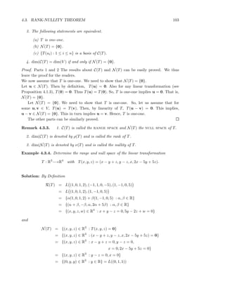
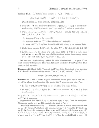
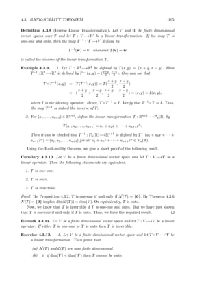
![106 CHAPTER 4. LINEAR TRANSFORMATIONS
ii. if dim(V ) > dim(W) then T cannot be one-one.
2. Let V be a vector space of dimension n and let B = (v1, . . . , vn) be an ordered basis of
V . For i = 1, . . . , n, let wi ∈ V with [wi]B = [a1i, a2i, . . . , ani ]t. Also, let A = [aij].
Then prove that w1, . . . , wn is a basis of V if and only if A is invertible.
3. Let T, S : V −→V be linear transformations with dim(V ) = n.
(a) Show that C(T + S) ⊂ C(T) + C(S). Deduce that ρ(T + S) ≤ ρ(T) + ρ(S).
(b) Now, use Theorem 4.3.6 to prove ν(T + S) ≥ ν(T) + ν(S) − n.
4. Let z1, z2, . . . , zk be k distinct complex numbers and define a linear transformation T :
Pn(C) −→ Ck by T P(z) = P(z1), P(z2), . . . , P(zk) . For each k ≥ 1, determine
dim(C(T)).
5. Fix A ∈ Mn(R) satisfying A2 = A and define TA : Rn −→ Rn by TA(vt) = Av, for
all vt ∈ Rn. Then prove that
(a) TA ◦ TA = TA. Equivalently, TA ◦ (I − TA) = 0, where I : Rn −→ Rn is the
identity map and 0 : Rn −→ Rn is the zero map.
(b) N(TA) ∩ C(TA) = {0}.
(c) Rn = C(TA) + N(TA). [Hint: x = TA(x) + (I − TA)(x)]
4.4 Similarity of Matrices
Let V be a finite dimensional vector space with ordered basis B. Then we saw that any
linear operator T : V −→V corresponds to a square matrix of order dim(V ) and this matrix
was denoted by T[B, B]. In this section, we will try to understand the relationship between
T[B1, B1] and T[B2, B2], where B1 and B2 are distinct ordered bases of V . This will enable
us to understand the reason for defining the matrix product somewhat differently.
Theorem 4.4.1 (Composition of Linear Transformations). Let V, W and Z be finite
dimensional vector spaces with ordered bases B1, B2 and B3, respectively. Also, let T :
V −→W and S : W−→Z be linear transformations. Then the composition map S ◦ T :
V −→Z (see Figure 4.2) is a linear transformation and
(V, B1, n) (W, B2, m) (Z, B3, p)
T[B1, B2]m×n S[B2, B3]p×m
(S ◦ T)[B1, B3]p×n = S[B2, B3] · T[B1, B2]
Figure 4.2: Composition of Linear Transformations
(S ◦ T) [B1, B3] = S[B2, B3] · T[B1, B2].](https://image.slidesharecdn.com/booklinear-160914134339/85/Book-linear-106-320.jpg)
![4.4. SIMILARITY OF MATRICES 107
Proof. Let B1 = (u1, . . . , un), B2 = (v1, . . . , vm) and B3 = (w1, . . . , wp) be ordered bases
of V, W and Z, respectively. Then using Equation (4.2.4), we have
(S ◦ T) (ut) = S(T(ut)) = S
m
j=1
(T[B1, B2])jtvj =
m
j=1
(T[B1, B2])jtS(vj)
=
m
j=1
(T[B1, B2])jt
p
k=1
(S[B2, B3])kjwk =
p
k=1
(
m
j=1
(S[B2, B3])kj(T[B1, B2])jt)wk
=
p
k=1
(S[B2, B3] T[B1, B2])ktwk.
Thus, using matrix multiplication, the t-th column of (S ◦ T) [B1, B3] is given by
[(S ◦ T) (ut)]B3 =
S[B2, B3] T[B1, B2] 1t
S[B2, B3] T[B1, B2] 2t
...
S[B2, B3] T[B1, B2] pt
= S[B2, B3]
T[B1, B2]1t
T[B1, B2]2t
...
T[B1, B2]pt
.
Hence, (S ◦ T)[B1, B3] = [(S ◦ T)(u1)]B3 , . . . , [(S ◦ T)(un)]B3 = S[B2, B3] · T[B1, B2] and
the proof of the theorem is over.
Proposition 4.4.2. Let V be a finite dimensional vector space and let T, S : V −→V be
two linear operators. Then ν(T) + ν(S) ≥ ν(T ◦ S) ≥ max{ν(T), ν(S)}.
Proof. We first prove the second inequality.
Suppose v ∈ N(S). Then (T ◦ S)(v) = T(S(v) = T(0) = 0 gives N(S) ⊂ N(T ◦ S).
Therefore, ν(S) ≤ ν(T ◦ S).
We now use Theorem 4.3.6 to see that the inequality ν(T) ≤ ν(T ◦ S) is equivalent to
showing C(T ◦ S) ⊂ C(T). But this holds true as C(S) ⊂ V and hence T(C(S)) ⊂ T(V ).
Thus, the proof of the second inequality is over.
For the proof of the first inequality, assume that k = ν(S) and {v1, . . . , vk} is a basis
of N(S). Then {v1, . . . , vk} ⊂ N(T ◦ S) as T(0) = 0. So, let us extend it to get a basis
{v1, . . . , vk, u1, . . . , uℓ} of N(T ◦ S).
Claim: {S(u1), S(u2), . . . , S(uℓ)} is a linearly independent subset of N(T).
It is easily seen that {S(u1), . . . , S(uℓ)} is a subset of N(T). So, let us solve the linear
system c1S(u1) + c2S(u2) + · · · + cℓS(uℓ) = 0 in the unknowns c1, c2, . . . , cℓ. This system
is equivalent to S(c1u1 + c2u2 + · · · + cℓuℓ) = 0. That is,
ℓ
i=1
ciui ∈ N(S). Hence,
ℓ
i=1
ciui
is a unique linear combination of the vectors v1, . . . , vk. Thus,
c1u1 + c2u2 + · · · + cℓuℓ = α1v1 + α2v2 + · · · + αkvk (4.4.1)
for some scalars α1, α2, . . . , αk. But by assumption, {v1, . . . , vk, u1, . . . , uℓ} is a basis of
N(T ◦ S) and hence linearly independent. Therefore, the only solution of Equation (4.4.1)
is given by ci = 0 for 1 ≤ i ≤ ℓ and αj = 0 for 1 ≤ j ≤ k.
Thus, {S(u1), S(u2), . . . , S(uℓ)} is a linearly independent subset of N(T) and so ν(T) ≥
ℓ. Hence, ν(T ◦ S) = k + ℓ ≤ ν(S) + ν(T).](https://image.slidesharecdn.com/booklinear-160914134339/85/Book-linear-107-320.jpg)
![108 CHAPTER 4. LINEAR TRANSFORMATIONS
Remark 4.4.3. Using Theorem 4.3.6 and Proposition 4.4.2, we see that if A and B are
two n × n matrices then
min{ρ(A), ρ(B)} ≥ ρ(AB) ≥ n − ρ(A) − ρ(B).
Let V be a finite dimensional vector space and let T : V −→V be an invertible linear
operator. Then using Theorem 4.3.7, the map T−1 : V −→V is a linear operator defined
by T−1(u) = v whenever T(v) = u. The next result relates the matrix of T and T−1. The
reader is required to supply the proof (use Theorem 4.4.1).
Theorem 4.4.4 (Inverse of a Linear Transformation). Let V be a finite dimensional vector
space with ordered bases B1 and B2. Also let T : V −→V be an invertible linear operator.
Then the matrix of T and T−1 are related by T[B1, B2]−1 = T−1[B2, B1].
Exercise 4.4.5. Find the matrix of the linear transformations given below.
1. Define T : R3−→R3 by T(1, 1, 1) = (1, −1, 1), T(1, −1, 1) = (1, 1, −1) and T(1, 1, −1) =
(1, 1, 1). Find T[B, B], where B = (1, 1, 1), (1, −1, 1), (1, 1, −1) . Is T an invertible
linear operator?
2. Let B = 1, x, x2, x3 be an ordered basis of P3(R). Define T : P3(R)−→P3(R) by
T(1) = 1, T(x) = 1 + x, T(x2
) = (1 + x)2
and T(x3
) = (1 + x)3
.
Prove that T is an invertible linear operator. Also, find T[B, B] and T−1[B, B].
We end this section with definition, results and examples related with the notion of
isomorphism. The result states that for each fixed positive integer n, every real vector
space of dimension n is isomorphic to Rn and every complex vector space of dimension n
is isomorphic to Cn.
Definition 4.4.6 (Isomorphism). Let V and W be two vector spaces over F. Then V
is said to be isomorphic to W if there exists a linear transformation T : V −→W that is
one-one, onto and invertible. We also denote it by V ∼= W.
Theorem 4.4.7. Let V be a vector space over R. If dim(V ) = n then V ∼= Rn.
Proof. Let B be the standard ordered basis of Rn and let B1 = v1, . . . , vn be an ordered
basis of V . Define a map T : V −→Rn by T(vi) = ei for 1 ≤ i ≤ n. Then it can be easily
verified that T is a linear transformation that is one-one, onto and invertible (the image of
a basis vector is a basis vector). Hence, the result follows.
A similar idea leads to the following result and hence we omit the proof.
Theorem 4.4.8. Let V be a vector space over C. If dim(V ) = n then V ∼= Cn.
Example 4.4.9. 1. The standard ordered basis of Pn(C) is given by 1, x, x2, . . . , xn .
Hence, define T : Pn(C)−→Cn+1 by T(xi) = ei+1 for 0 ≤ i ≤ n. In general, verify
that T(a0 + a1x + · · · + anxn) = (a0, a1, . . . , an) and T is linear transformation which
is one-one, onto and invertible. Thus, the vector space Pn(C) ∼= Cn+1.](https://image.slidesharecdn.com/booklinear-160914134339/85/Book-linear-108-320.jpg)
![4.5. CHANGE OF BASIS 109
2. Let V = {(x, y, z, w) ∈ R4 : x − y + z − w = 0}. Suppose that B is the standard
ordered basis of R3 and B1 = (1, 1, 0, 0), (−1, 0, 1, 0), (1, 0, 0, 1) is the ordered basis
of V . Then T : V −→R3 defined by T(v) = T(y −z +w, y, z, w) = (y, z, w) is a linear
transformation and T[B1, B] = I3. Thus, T is one-one, onto and invertible.
4.5 Change of Basis
Let V be a vector space with ordered bases B1 = (u1, . . . , un) and B2 = (v1, . . . , vn}. Also,
recall that the identity linear operator I : V −→V is defined by I(x) = x for every x ∈ V.
If
I[B2, B1] = [I(v1)]B1 , [I(v2)]B1 , . . . , [I(vn)]B1 =
a11 a12 · · · a1n
a21 a22 · · · a2n
...
...
...
...
an1 an2 · · · ann
then by definition of I[B2, B1], we see that vi = I(vi) =
n
j=1
ajiuj for all i, 1 ≤ i ≤ n. Thus,
we have proved the following result which also appeared in another form in Theorem 3.4.5.
Theorem 4.5.1 (Change of Basis Theorem). Let V be a finite dimensional vector space
with ordered bases B1 = (u1, u2, . . . , un} and B2 = (v1, v2, . . . , vn}. Suppose x ∈ V with
[x]B1 = (α1, α2, . . . , αn)t and [x]B2 = (β1, β2, . . . , βn)t. Then [x]B1 = I[B2, B1] [x]B2 . Or
equivalently,
α1
α2
...
αn
=
a11 a12 · · · a1n
a21 a22 · · · a2n
...
...
...
...
an1 an2 · · · ann
β1
β2
...
βn
.
Remark 4.5.2. Observe that the identity linear operator I : V −→V is invertible and
hence by Theorem 4.4.4 I[B2, B1]−1 = I−1[B1, B2] = I[B1, B2]. Therefore, we also have
[x]B2 = I[B1, B2] [x]B1 .
Let V be a finite dimensional vector space with ordered bases B1 and B2. Then for any
linear operator T : V −→V the next result relates T[B1, B1] and T[B2, B2].
Theorem 4.5.3. Let B1 = (u1, . . . , un) and B2 = (v1, . . . , vn) be two ordered bases of a
vector space V . Also, let A = [aij] = I[B2, B1] be the matrix of the identity linear operator.
Then for any linear operator T : V −→V
T[B2, B2] = A−1
· T[B1, B1] · A = I[B1, B2] · T[B1, B1] · I[B2, B1]. (4.5.2)
Proof. The proof uses Theorem 4.4.1 by representing T[B1, B2] as (I ◦ T)[B1, B2] and (T ◦
I)[B1, B2], where I is the identity operator on V (see Figure 4.3). By Theorem 4.4.1, we
have
T[B1, B2] = (I ◦ T)[B1, B2] = I[B1, B2] · T[B1, B1]
= (T ◦ I)[B1, B2] = T[B2, B2] · I[B1, B2].](https://image.slidesharecdn.com/booklinear-160914134339/85/Book-linear-109-320.jpg)
![110 CHAPTER 4. LINEAR TRANSFORMATIONS
(V, B1) (V, B1)
(V, B2) (V, B2)
T[B1, B1]
T[B2, B2]
I[B1, B2] I[B1, B2]
T ◦ I
I ◦ T
Figure 4.3: Commutative Diagram for Similarity of Matrices
Thus, using I[B2, B1] = I[B1, B2]−1, we get I[B1, B2] T[B1, B1] I[B2, B1] = T[B2, B2] and
the result follows.
Let T : V −→V be a linear operator on V . If dim(V ) = n then each ordered basis B of
V gives rise to an n × n matrix T[B, B]. Also, we know that for any vector space we have
infinite number of choices for an ordered basis. So, as we change an ordered basis, the
matrix of the linear transformation changes. Theorem 4.5.3 tells us that all these matrices
are related by an invertible matrix (see Remark 4.5.2). Thus we are led to the following
remark and the definition.
Remark 4.5.4. The Equation (4.5.2) shows that T[B2, B2] = I[B1, B2]·T[B1, B1]·I[B2, B1].
Hence, the matrix I[B1, B2] is called the B1 : B2 change of basis matrix.
Definition 4.5.5 (Similar Matrices). Two square matrices B and C of the same order
are said to be similar if there exists a non-singular matrix P such that P−1BP = C or
equivalently BP = PC.
Example 4.5.6. 1. Let B1 = 1 + x, 1 + 2x + x2, 2 + x and B2 = 1, 1 + x, 1 + x + x2
be ordered bases of P2(R). Then I(a + bx + cx2) = a + bx + cx2. Thus,
I[B2, B1] = [[1]B1 , [1 + x]B1 , [1 + x + x2
]B1 ] =
−1 1 −2
0 0 1
1 0 1
and
I[B1, B2] = [[1 + x]B2 , [1 + 2x + x2
]B2 , [2 + x]B2 ] =
0 −1 1
1 1 1
0 1 0
.
Also, verify that I[B1, B2]−1 = I[B2, B1].
2. Let B1 = (1, 0, 0), (1, 1, 0), (1, 1, 1) and B2 = 1, 1, −1), (1, 2, 1), (2, 1, 1) be two
ordered bases of R3. Define T : R3−→R3 by T(x, y, z) = (x + y, x + y + 2z, y − z).
Then T[B1, B1] =
0 0 −2
1 1 4
0 1 0
and T[B2, B2] =
−4/5 1 8/5
−2/5 2 9/5
8/5 0 −1/5
. Also, check that](https://image.slidesharecdn.com/booklinear-160914134339/85/Book-linear-110-320.jpg)
![4.6. SUMMARY 111
I[B2, B1] =
0 −1 1
2 1 0
−1 1 1
and
T[B1, B1] I[B2, B1] = I[B2, B1] T[B2, B2] =
2 −2 −2
−2 4 5
2 1 0
.
Exercise 4.5.7. 1. Let V be an n-dimensional vector space and let T : V −→V be a
linear operator. Suppose T has the property that Tn−1 = 0 but Tn = 0.
(a) Prove that there exists u ∈ V with {u, T(u), . . . , Tn−1(u)}, a basis of V.
(b) For B = u, T(u), . . . , Tn−1(u) prove that T[B, B] =
0 0 0 · · · 0
1 0 0 · · · 0
0 1 0 · · · 0
...
...
...
...
0 0 · · · 1 0
.
(c) Let A be an n × n matrix satisfying An−1 = 0 but An = 0. Then prove that A
is similar to the matrix given in Part 1b.
2. Define T : R3−→R3 by T(x, y, z) = (x + y + 2z, x − y − 3z, 2x + 3y + z). Let B be the
standard basis and B1 = (1, 1, 1), (1, −1, 1), (1, 1, 2) be another ordered basis of R3.
Then find the
(a) matrices T[B, B] and T[B1, B1].
(b) matrix P such that P−1T[B, B] P = T[B1, B1].
3. Define T : R3−→R3 by T(x, y, z) = (x, x + y, x + y + z). Let B be the standard basis
and B1 = (1, 0, 0), (1, 1, 0), (1, 1, 1) be another ordered basis of R3. Then find the
(a) matrices T[B, B] and T[B1, B1].
(b) matrix P such that P−1T[B, B] P = T[B1, B1].
4. Let B1 = (1, 2, 0), (1, 3, 2), (0, 1, 3) and B2 = (1, 2, 1), (0, 1, 2), (1, 4, 6) be two or-
dered bases of R3. Find the change of basis matrix
(a) P from B1 to B2.
(b) Q from B2 to B1.
(c) from the standard basis of R3 to B1. What do you notice?
Is it true that PQ = I = QP? Give reasons for your answer.
4.6 Summary](https://image.slidesharecdn.com/booklinear-160914134339/85/Book-linear-111-320.jpg)

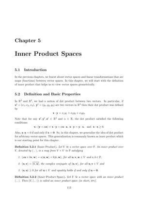
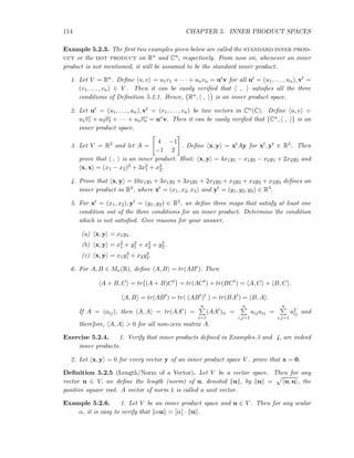
![5.2. DEFINITION AND BASIC PROPERTIES 115
2. Let ut = (1, −1, 2, −3) ∈ R4. Then u =
√
1 + 1 + 4 + 9 =
√
15. Thus, 1√
15
u and
− 1√
15
u are vectors of norm 1 in the vector subspace L(u) of R4. Or equivalently,
1√
15
u is a unit vector in the direction of u.
Exercise 5.2.7. 1. Let ut = (−1, 1, 2, 3, 7) ∈ R5. Find all α ∈ R such that αu = 1.
2. Let ut = (−1, 1, 2, 3, 7) ∈ C5. Find all α ∈ C such that αu = 1.
3. Prove that x + y 2 + x − y 2 = 2 x 2 + y 2 , for all x, y ∈ Rn. This equality
is commonly known as the Parallelogram Law as in a parallelogram the sum of
square of the lengths of the diagonals equals twice the sum of squares of the lengths
of the sides.
4. Prove that for any two continuous functions f(x), g(x) ∈ C([−1, 1]), the map f(x), g(x) =
1
−1 f(x) · g(x)dx defines an inner product in C([−1, 1]).
5. Fix an ordered basis B = (u1, . . . , un) of a complex vector space V . Prove that ,
defined by u, v =
n
i=1
aibi, whenever [u]B = (a1, . . . , an)t and [v]B = (b1, . . . , bn)t is
indeed an inner product in V .
A very useful and a fundamental inequality concerning the inner product is due to
Cauchy and Schwarz. The next theorem gives the statement and a proof of this inequality.
Theorem 5.2.8 (Cauchy-Bunyakovskii-Schwartz inequality). Let V (F) be an inner product
space. Then for any u, v ∈ V
| u, v | ≤ u v . (5.2.1)
Equality holds in Equation (5.2.1) if and only if the vectors u and v are linearly dependent.
Furthermore, if u = 0, then in this case v = v,
u
u
u
u
.
Proof. If u = 0, then the inequality (5.2.1) holds trivially. Hence, let u = 0. Also, by
the third property of inner product, λu + v, λu + v ≥ 0 for all λ ∈ F. In particular, for
λ = −
v, u
u 2
,
0 ≤ λu + v, λu + v = λλ u 2
+ λ u, v + λ v, u + v 2
=
v, u
u 2
v, u
u 2
u 2
−
v, u
u 2
u, v −
v, u
u 2
v, u + v 2
= v 2
−
| v, u |2
u 2
.
Or, in other words | v, u |2 ≤ u 2 v 2 and the proof of the inequality is over.
If u = 0 then λu + v, λu + v = 0 if and only of λu + v = 0. Hence, equality holds
in (5.2.1) if and only if λ = −
v, u
u 2
. That is, u and v are linearly dependent and in this
case v = v, u
u
u
u .](https://image.slidesharecdn.com/booklinear-160914134339/85/Book-linear-115-320.jpg)
![116 CHAPTER 5. INNER PRODUCT SPACES
Let V be a real vector space. Then for every u, v ∈ V, the Cauchy-Schwarz inequality
(see (5.2.1)) implies that −1 ≤ u,v
u v ≤ 1. Also, we know that cos : [0, π] −→ [−1, 1]
is an one-one and onto function. We use this idea, to relate inner product with the angle
between two vectors in an inner product space V .
Definition 5.2.9 (Angle between two vectors). Let V be a real vector space and let u, v ∈
V . Suppose θ is the angle between u, v. We define
cos θ =
u, v
u v
.
1. The real number θ, with 0 ≤ θ ≤ π, and satisfying cos θ =
u, v
u v
is called the angle
between the two vectors u and v in V.
Definition 5.2.10 (Orthogonal Vectors). Let V be a vector space.
1. The vectors u and v in V are said to be orthogonal if u, v = 0. Orthogonality
corresponds to perpendicularity.
2. A set of vectors {u1, u2, . . . , un} in V is called mutually orthogonal if ui, uj = 0
for all 1 ≤ i = j ≤ n.
a
b
c
A B
C
Figure 2: Triangle with vertices A, B and C
Before proceeding further with one more definition, recall that if ABC are vertices of
a triangle (see Figure 5.2) then cos(A) = b2+c2−a2
2bc . We prove this as our next result.
Lemma 5.2.11. Let A, B and C be the sides of a triangle in a real inner product space V
then
cos(A) =
b2 + c2 − a2
2bc
.
Proof. Let the coordinates of the vertices A, B and C be 0, u and v, respectively. Then
AB = u, AC = v and BC = v − u. Thus, we need to prove that
cos(A) =
v 2 + u 2 − v − u 2
2 v u
.
Now, using the properties of an inner product and Definition 5.2.9, it follows that
v 2
+ u 2
− v − u 2
= 2 u, v = 2 v u cos(A).
Thus, the required result follows.](https://image.slidesharecdn.com/booklinear-160914134339/85/Book-linear-116-320.jpg)
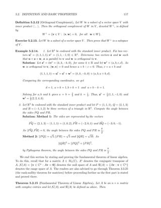
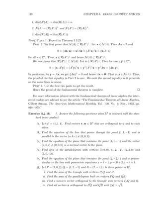
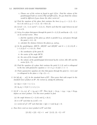
![120 CHAPTER 5. INNER PRODUCT SPACES
[Hint: Consider a symmetric matrix A =
a b
b c
. Define x, y = ytAx. Use the
given conditions to get a linear system of 3 equations in the unknowns a, b, c. Solve
this system.]
5. Let W = {(x, y, z) ∈ R3 : x + y + z = 0}. Find a basis of W⊥.
6. Let W be a subspace of a finite dimensional inner product space V . Prove that
(W⊥)⊥ = W.
7. Let xt = (x1, x2, x3), yt = (y1, y2, y3) ∈ R3. Show that
x, y = 10x1y1 + 3x1y2 + 3x2y1 + 4x2y2 + x2y3 + x3y2 + 3x3y3
is an inner product in R3(R). With respect to this inner product, find the angle between
the vectors (1, 1, 1) and (2, −5, 2).
8. Recall the inner product space Mn×n(R) (see Example 5.2.3.6). Determine W⊥ for
the subspace W = {A ∈ Mn×n(R) : At = A}.
9. Prove that f(x), g(x) =
π
−π
f(x) · g(x)dx defines an inner product in C[−π, π].
Define 1(x) = 1 for all x ∈ [−π, π]. Prove that
S = {1} ∪ {cos(mx) : m ≥ 1} ∪ {sin(nx) : n ≥ 1}
is a linearly independent subset of C[−π, π].
10. Let V be an inner product space. Prove the triangle inequality
u + v ≤ u + v for every u, v ∈ V.
11. Let z1, z2, . . . , zn ∈ C. Use the Cauchy-Schwarz inequality to prove that
|z1 + z2 + · · · + zn| ≤ n(|z1|2 + |z2|2 + · · · + |zn|2).
When does the equality hold?
12. Let x, y ∈ Rn. Prove the following:
(a) x, y = 0 ⇐⇒ x − y 2 = x 2 + y 2 (Pythagoras Theorem).
(b) x = y ⇐⇒ x + y, x − y = 0 (x and y form adjacent sides of a rhombus
as the diagonals x + y and x − y are orthogonal).
(c) 4 x, y = x + y 2 − x − y 2 (polarization identity).
Are the above results true if x, y ∈ Cn(C)?
13. Let x, y ∈ Cn(C). Prove that
(a) 4 x, y = x + y 2 − x − y 2 + i x + iy 2 − i x − iy 2.](https://image.slidesharecdn.com/booklinear-160914134339/85/Book-linear-120-320.jpg)
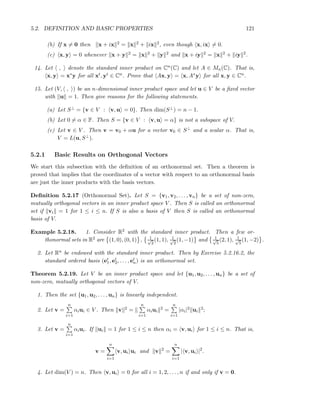
![122 CHAPTER 5. INNER PRODUCT SPACES
Proof. Consider the linear system
c1u1 + c2u2 + · · · + cnun = 0 (5.2.2)
in the unknowns c1, c2, . . . , cn. As 0, u = 0 for each u ∈ V and uj, ui = 0 for all j = i,
we have
0 = 0, ui = c1u1 + c2u2 + · · · + cnun, ui =
n
j=1
cj uj, ui = ci ui, ui .
As ui = 0, ui, ui = 0 and therefore ci = 0 for 1 ≤ i ≤ n. Thus, the linear system (5.2.2)
has only the trivial solution. Hence, the proof of Part 1 is complete.
For Part 2, we use a similar argument to get
n
i=1
αiui
2
=
n
i=1
αiui,
n
i=1
αiui =
n
i=1
αi ui,
n
j=1
αjuj
=
n
i=1
αi
n
j=1
αj ui, uj =
n
i=1
αiαi ui, ui =
n
i=1
|αi|2
ui
2
.
Note that v, ui = n
j=1 αjuj, ui = n
j=1 αj uj, ui = αj. Thus, the proof of Part 3
is complete.
Part 4 directly follows using Part 3 as the set {u1, u2, . . . , un} is a basis of V. Therefore,
we have obtained the required result.
In view of Theorem 5.2.19, we inquire into the question of extracting an orthonormal
basis from a given basis. In the next section, we describe a process (called the Gram-
Schmidt Orthogonalization process) that generates an orthonormal set from a given set
containing finitely many vectors.
Remark 5.2.20. The last two parts of Theorem 5.2.19 can be rephrased as follows:
Let B = v1, . . . , vn be an ordered orthonormal basis of an inner product space V and let
u ∈ V . Then
[u]B = ( u, v1 , u, v2 , . . . , u, vn )t
.
Exercise 5.2.21. 1. Let B = 1√
2
(1, 1), 1√
2
(1, −1) be an ordered basis of R2. Deter-
mine [(2, 3)]B. Also, compute [(x, y)]B.
2. Let B = 1√
3
(1, 1, 1), 1√
2
(1, −1, 0), 1√
6
(1, 1, −2), be an ordered basis of R3. Determine
[(2, 3, 1)]B. Also, compute [(x, y, z)]B.
3. Let ut = (u1, u2, u3), vt = (v1, v2, v3) be two vectors in R3. Then recall that their
cross product, denoted u × v, equals
ut
× vt
= (u2v3 − u3v2, u3v1 − u1v3, u1v2 − u2v1).
Use this to find an orthonormal basis of R3 containing the vector 1√
6
(1, 2, 1).](https://image.slidesharecdn.com/booklinear-160914134339/85/Book-linear-122-320.jpg)
![5.3. GRAM-SCHMIDT ORTHOGONALIZATION PROCESS 123
4. Let ut = (1, −1, −2). Find vectors vt, wt ∈ R3 such that v and w are orthogonal to
u and to each other as well.
5. Let A be an n × n orthogonal matrix. Prove that the rows/columns of A form an
orthonormal basis of Rn.
6. Let A be an n × n unitary matrix. Prove that the rows/columns of A form an or-
thonormal basis of Cn.
7. Let {ut
1, ut
2, . . . , ut
n} be an orthonormal basis of Rn. Prove that the n × n matrix
A = [u1, u2, . . . , un] is an orthogonal matrix.
5.3 Gram-Schmidt Orthogonalization Process
Suppose we are given two non-zero vectors u and v in a plane. Then in many instances, we
need to decompose the vector v into two components, say y and z, such that y is a vector
parallel to u and z is a vector perpendicular (orthogonal) to u. We do this as follows (see
Figure 5.3):
Let ˆu =
u
u
. Then ˆu is a unit vector in the direction of u. Also, using trigonometry, we
know that cos(θ) = OQ
OP
and hence OQ = OP cos(θ). Or using Definition 5.2.9,
OQ = v
v, u
v u
=
v, u
u
,
where we need to take the absolute value of the right hand side expression as the length
of a vector is always a positive quantity. Thus, we get
OQ = OQ ˆu = v,
u
u
u
u
.
Thus, we see that y = OQ = v, u
u
u
u and z = v − v, u
u
u
u . It is easy to verify that
v = y + z, y is parallel to u and z is orthogonal to u. In literature, the vector y = OQ
is often called the orthogonal projection of the vector v on u and is denoted by Proju(v).
Thus,
Proju(v) = v,
u
u
u
u
and Proju(v) = OQ =
v, u
u
. (5.3.1)
Moreover, the distance of the vector u from the point P equals OR = PQ =
v − v, u
u
u
u .
OR = v − v,u
u 2 u OQ = v,u
u 2 u
R
θO
Q
P
u
v
Figure 3: Decomposition of vector v](https://image.slidesharecdn.com/booklinear-160914134339/85/Book-linear-123-320.jpg)
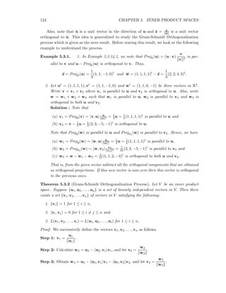
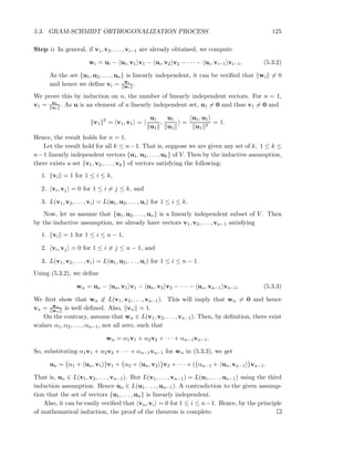
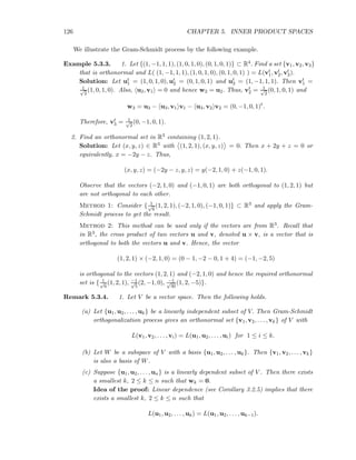
![5.3. GRAM-SCHMIDT ORTHOGONALIZATION PROCESS 127
Also, by Gram-Schmidt orthogonalization process
L(u1, u2, . . . , uk−1) = L(v1, v2, . . . , vk−1).
Thus, uk ∈ L(v1, v2, . . . , vk−1) and hence by Remark 5.2.20
uk = uk, v1 v1 + uk, v2 v2 + · · · + uk, vk−1 vk−1.
So, by definition wk = 0.
2. Let S be a countably infinite set of linearly independent vectors. Then one can apply
the Gram-Schmidt process to get a countably infinite orthonormal set.
3. Consider Rn with the standard inner product and let {v1, v2, . . . , vn} be an orthonor-
mal set. Then, we see that
(a) vi = 1 is equivalent to vt
ivi = 1, for 1 ≤ i ≤ n,
(b) vi, vj = 0 is equivalent to vt
ivj = 0, for 1 ≤ i = j ≤ n.
Hence, we see that
At
A =
vt
1
vt
2
...
vt
n
[v1, v2, . . . , vn]
=
vt
1v1 vt
1v2 · · · vt
1vn
vt
2v1 vt
2v2 · · · vt
2vn
...
...
...
...
vt
nv1 vt
nv2 · · · vt
nvn
=
1 0 · · · 0
0 1 · · · 0
...
...
...
...
0 0 · · · 1
= In.
Since AtA = In, it follows that AAt = In. But,
AAt
= [v1, v2, . . . , vn]
vt
1
vt
2
...
vt
n
= v1vt
1 + v2vt
2 + · · · + vnvt
n.
Now, for each i, 1 ≤ i ≤ n, the matrix vivt
i has the following properties:
(a) it is symmetric;
(b) it is idempotent; and
(c) it has rank one.
4. The first two properties imply that the matrix vivt
i, for each i, 1 ≤ i ≤ n is a projection
operator. That is, the identity matrix is the sum of projection operators, each of rank
1.
5. Now define a linear transformation T : Rn−→Rn by T(x) = (vivt
i)x = (vt
ix)vi is a
projection operator on the subspace L(vi).](https://image.slidesharecdn.com/booklinear-160914134339/85/Book-linear-127-320.jpg)
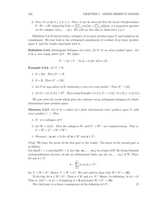
![5.3. GRAM-SCHMIDT ORTHOGONALIZATION PROCESS 129
Exercise 5.3.8. 1. Let A be an n × n orthogonal matrix. Then prove that
(a) the rows of A form an orthonormal basis of Rn.
(b) the columns of A form an orthonormal basis of Rn.
(c) for any two vectors x, y ∈ Rn×1, Ax, Ay = x, y .
(d) for any vector x ∈ Rn×1, Ax = x .
2. Let A be an n × n unitary matrix. Then prove that
(a) the rows/columns of A form an orthonormal basis of the complex vector space
Cn.
(b) for any two vectors x, y ∈ Cn×1, Ax, Ay = x, y .
(c) for any vector x ∈ Cn×1, Ax = x .
3. Let A and B be two n × n orthogonal matrices. Then prove that AB and BA are
both orthogonal matrices. Prove a similar result for unitary matrices.
4. Prove the statements made in Remark 5.3.4.3 about orthogonal matrices. State and
prove a similar result for unitary matrices.
5. Let A be an n × n upper triangular matrix. If A is also an orthogonal matrix then A
is a diagonal matrix with diagonal entries ±1.
6. Determine an orthonormal basis of R4 containing the vectors (1, −2, 1, 3) and (2, 1, −3, 1).
7. Consider the real inner product space C[−1, 1] with f, g =
1
−1
f(t)g(t)dt. Prove that
the polynomials 1, x, 3
2x2 − 1
2, 5
2x3 − 3
2x form an orthogonal set in C[−1, 1]. Find the
corresponding functions f(x) with f(x) = 1.
8. Consider the real inner product space C[−π, π] with f, g =
π
−π
f(t)g(t)dt. Find an
orthonormal basis for L (x, sin x, sin(x + 1)) .
9. Let M be a subspace of Rn and dim M = m. A vector x ∈ Rn is said to be orthogonal
to M if x, y = 0 for every y ∈ M.
(a) How many linearly independent vectors can be orthogonal to M?
(b) If M = {(x1, x2, x3) ∈ R3 : x1 + x2 + x3 = 0}, determine a maximal set of
linearly independent vectors orthogonal to M in R3.
10. Determine an orthogonal basis of L ({(1, 1, 0, 1), (−1, 1, 1, −1), (0, 2, 1, 0), (1, 0, 0, 0)})
in R4.
11. Let Rn be endowed with the standard inner product. Suppose we have a vector xt =
(x1, x2, . . . , xn) ∈ Rn with x = 1.](https://image.slidesharecdn.com/booklinear-160914134339/85/Book-linear-129-320.jpg)
![130 CHAPTER 5. INNER PRODUCT SPACES
(a) Then prove that the set {x} can always be extended to form an orthonormal
basis of Rn.
(b) Let this basis be {x, x2, . . . , xn}. Suppose B = (e1, e2, . . . , en) is the standard
basis of Rn and let A = [x]B, [x2]B, . . . , [xn]B . Then prove that A is an
orthogonal matrix.
12. Let v, w ∈ Rn, n ≥ 1 with u = w = 1. Prove that there exists an orthogonal
matrix A such that Av = w. Prove also that A can be chosen such that det(A) = 1.
5.4 Orthogonal Projections and Applications
Recall that given a k-dimensional vector subspace of a vector space V of dimension n, one
can always find an (n − k)-dimensional vector subspace W0 of V (see Exercise 3.3.13.5)
satisfying
W + W0 = V and W ∩ W0 = {0}.
The subspace W0 is called the complementary subspace of W in V. We first use Theo-
rem 5.3.7 to get the complementary subspace in such a way that the vectors in different
subspaces are orthogonal. That is, w, v = 0 for all w ∈ W and v ∈ W0. We then use this
to define an important class of linear transformations on an inner product space, called
orthogonal projections.
Definition 5.4.1 (Orthogonal Complement and Orthogonal Projection). Let W be a sub-
space of a finite dimensional inner product space V .
1. Then W⊥ is called the orthogonal complement of W in V. We represent it by writing
V = W ⊕ W⊥ in place of V = W + W⊥.
2. Also, for each v ∈ V there exist unique vectors w ∈ W and u ∈ W⊥ such that
v = w + u. We use this to define
PW : V −→ V by PW (v) = w.
Then PW is called the orthogonal projection of V onto W.
Exercise 5.4.2. Let W be a subspace of a finite dimensional inner product space V . Use
V = W ⊕ W⊥ to define the orthogonal projection operator PW ⊥ of V onto W⊥. Prove
that the maps PW and PW ⊥ are indeed linear transformations. What can you say about
PW + PW ⊥ ?
Example 5.4.3. 1. Let V = R3 and W = {(x, y, z) ∈ R3 : x + y − z = 0}. Then it can
be easily verified that {(1, 1, −1)} is a basis of W⊥ as for each (x, y, z) ∈ W, we have
x + y − z = 0 and hence
(x, y, z), (1, 1, −1) = x + y − z = 0 for each (x, y, z) ∈ W.](https://image.slidesharecdn.com/booklinear-160914134339/85/Book-linear-130-320.jpg)
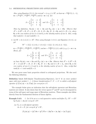
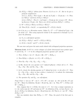
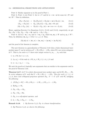
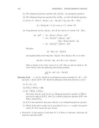
![5.4. ORTHOGONAL PROJECTIONS AND APPLICATIONS 135
5.4.1 Matrix of the Orthogonal Projection
The minimization problem stated above arises in lot of applications. So, it is very helpful
if the matrix of the orthogonal projection can be obtained under a given basis.
To this end, let W be a k-dimensional subspace of Rn with W⊥ as its orthogonal
complement. Let PW : Rn −→ Rn be the orthogonal projection of Rn onto W. Then
Remark 5.3.4.6 implies that we just need to know an orthonormal basis of W. So, let B =
(v1, v2, . . . , vk) be an orthonormal basis of W. Thus, the matrix of PW equals k
i=1 vivt
i.
Hence, we have proved the following theorem.
Theorem 5.4.10. Let W be a k-dimensional subspace of Rn and let PW be the corre-
sponding orthogonal projection of Rn onto W. Also assume that B = (v1, v2, . . . , vk) is
an orthonormal ordered basis of W. Define A = [v1, v2, . . . , vk], an n × k matrix. Then
the matrix of PW in the standard ordered basis of Rn is AAt = k
i=1 vivt
i (a symmetric
matrix).
We illustrate the above theorem with the help of an example. One can also see Exam-
ple 5.4.3.
Example 5.4.11. Let W = {(x, y, z, w) ∈ R4 : x = y, z = w} be a subspace of W.
Then an orthonormal ordered basis of W and W⊥ is 1√
2
(1, 1, 0, 0), 1√
2
(0, 0, 1, 1) and
1√
2
(1, −1, 0, 0), 1√
2
(0, 0, 1, −1) , respectively. Let PW : R4 −→ R4 be an orthogonal projec-
tion of R4 onto W. Then
A =
1√
2
0
1√
2
0
0 1√
2
0 1√
2
and PW [B, B] = AAt
=
1
2
1
2 0 0
1
2
1
2 0 0
0 0 1
2
1
2
0 0 1
2
1
2
,
where B = 1√
2
(1, 1, 0, 0), 1√
2
(0, 0, 1, 1), 1√
2
(1, −1, 0, 0), 1√
2
(0, 0, 1, −1) . Verify that
1. PW [B, B] is symmetric,
2. (PW [B, B])2
= PW [B, B] and
3. I4 − PW [B, B] PW [B, B] = 0 = PW [B, B] I4 − PW [B, B] .
Also, [(x, y, z, w)]B = x+y√
2
, z+w√
2
, x−y√
2
, z−w√
2
t
and hence
PW (x, y, z, w) =
x + y
2
(1, 1, 0, 0) +
z + w
2
(0, 0, 1, 1)
is the closest vector to the subspace W for any vector (x, y, z, w) ∈ R4.
Exercise 5.4.12. 1. Show that for any non-zero vector vt ∈ Rn, rank(vvt) = 1.
2. Let W be a subspace of an inner product space V and let P : V −→ V be the
orthogonal projection of V onto W. Let B be an orthonormal ordered basis of V.
Then prove that (P[B, B])t
= P[B, B].](https://image.slidesharecdn.com/booklinear-160914134339/85/Book-linear-135-320.jpg)
![136 CHAPTER 5. INNER PRODUCT SPACES
3. Let W1 = {(x, 0) : x ∈ R} and W2 = {(x, x) : x ∈ R} be two subspaces of R2. Let
PW1 and PW2 be the corresponding orthogonal projection operators of R2 onto W1
and W2, respectively. Compute PW1 ◦ PW2 and conclude that the composition of two
orthogonal projections need not be an orthogonal projection?
4. Let W be an (n−1)-dimensional subspace of Rn. Suppose B is an orthogonal ordered
basis of Rn obtained by extending an orthogonal ordered basis of W. Define
T : Rn
−→ Rn
by T(v) = w0 − w
whenever v = w + w0 for some w ∈ W and w0 ∈ W⊥. Then
(a) prove that T is a linear transformation,
(b) find T[B, B] and
(c) prove that T[B, B] is an orthogonal matrix.
T is called the reflection operator along W⊥.
5.5 QR Decomposition∗
The next result gives the proof of the QR decomposition for real matrices. A similar
result holds for matrices with complex entries. The readers are advised to prove that
for themselves. This decomposition and its generalizations are helpful in the numerical
calculations related with eigenvalue problems (see Chapter 6).
Theorem 5.5.1 (QR Decomposition). Let A be a square matrix of order n with real
entries. Then there exist matrices Q and R such that Q is orthogonal and R is upper
triangular with A = QR.
In case, A is non-singular, the diagonal entries of R can be chosen to be positive. Also,
in this case, the decomposition is unique.
Proof. We prove the theorem when A is non-singular. The proof for the singular case is
left as an exercise.
Let the columns of A be x1, x2, . . . , xn. Then {x1, x2, . . . , xn} is a basis of Rn and hence
the Gram-Schmidt orthogonalization process gives an ordered basis (see Remark 5.3.4), say
B = (v1, v2, . . . , vn) of Rn satisfying
L(v1, v2, . . . , vi) = L(x1, x2, . . . , xi),
vi = 1, vi, vj = 0,
for 1 ≤ i = j ≤ n. (5.5.4)
As xi ∈ Rn and xi ∈ L(v1, v2, . . . , vi), we can find αji, 1 ≤ j ≤ i such that
xi = α1iv1 + α2iv2 + · · · + αiivi = (α1i, . . . , αii, 0 . . . , 0)t
B
. (5.5.5)](https://image.slidesharecdn.com/booklinear-160914134339/85/Book-linear-136-320.jpg)
![5.5. QR DECOMPOSITION∗ 137
Now define Q = [v1, v2, . . . , vn] and R =
α11 α12 · · · α1n
0 α22 · · · α2n
...
...
...
...
0 0 · · · αnn
. Then by Exercise 5.3.8.4,
Q is an orthogonal matrix and using (5.5.5), we get
QR = [v1, v2, . . . , vn]
α11 α12 · · · α1n
0 α22 · · · α2n
...
...
...
...
0 0 · · · αnn
= α11v1, α12v1 + α22v2, . . . ,
n
i=1
αinvi
= [x1, x2, . . . , xn] = A.
Thus, we see that A = QR, where Q is an orthogonal matrix (see Remark 5.3.4.1) and R
is an upper triangular matrix.
The proof doesn’t guarantee that for 1 ≤ i ≤ n, αii is positive. But this can be achieved
by replacing the vector vi by −vi whenever αii is negative.
Uniqueness: suppose Q1R1 = Q2R2 then Q−1
2 Q1 = R2R−1
1 . Observe the following
properties of upper triangular matrices.
1. The inverse of an upper triangular matrix is also an upper triangular matrix, and
2. product of upper triangular matrices is also upper triangular.
Thus the matrix R2R−1
1 is an upper triangular matrix. Also, by Exercise 5.3.8.3, the matrix
Q−1
2 Q1 is an orthogonal matrix. Hence, by Exercise 5.3.8.5, R2R−1
1 = In. So, R2 = R1 and
therefore Q2 = Q1.
Let A = [x1, x2, . . . , xk] be an n × k matrix with rank (A) = r. Then by Remark
5.3.4.1c , the Gram-Schmidt orthogonalization process applied to {x1, x2, . . . , xk} yields a
set {v1, v2, . . . , vr} of orthonormal vectors of Rn and for each i, 1 ≤ i ≤ r, we have
L(v1, v2, . . . , vi) = L(x1, x2, . . . , xj), for some j, i ≤ j ≤ k.
Hence, proceeding on the lines of the above theorem, we have the following result.
Theorem 5.5.2 (Generalized QR Decomposition). Let A be an n × k matrix of rank r.
Then A = QR, where
1. Q = [v1, v2, . . . , vr] is an n × r matrix with QtQ = Ir,
2. L(v1, v2, . . . , vr) = L(x1, x2, . . . , xk), and
3. R is an r × k matrix with rank (R) = r.](https://image.slidesharecdn.com/booklinear-160914134339/85/Book-linear-137-320.jpg)
![138 CHAPTER 5. INNER PRODUCT SPACES
Example 5.5.3. 1. Let A =
1 0 1 2
0 1 −1 1
1 0 1 1
0 1 1 1
. Find an orthogonal matrix Q and an
upper triangular matrix R such that A = QR.
Solution: From Example 5.3.3, we know that
v1 =
1
√
2
(1, 0, 1, 0), v2 =
1
√
2
(0, 1, 0, 1) and v3 =
1
√
2
(0, −1, 0, 1). (5.5.6)
We now compute w4. If we denote u4 = (2, 1, 1, 1)t then
w4 = u4 − u4, v1 v1 − u4, v2 v2 − u4, v3 v3 =
1
2
(1, 0, −1, 0)t
. (5.5.7)
Thus, using Equations (5.5.6), (5.5.7) and Q = v1, v2, v3, v4 , we get
Q =
1√
2
0 0 1√
2
0 1√
2
−1√
2
0
1√
2
0 0 −1√
2
0 1√
2
1√
2
0
and R =
√
2 0
√
2 3√
2
0
√
2 0
√
2
0 0
√
2 0
0 0 0 −1√
2
. The readers are advised
to check that A = QR is indeed correct.
2. Let A =
1 1 1 0
−1 0 −2 1
1 1 1 0
1 0 2 1
. Find a 4 × 3 matrix Q satisfying QtQ = I3 and an upper
triangular matrix R such that A = QR.
Solution: Let us apply the Gram Schmidt orthogonalization process to the columns of
A. That is, apply the process to the subset {(1, −1, 1, 1), (1, 0, 1, 0), (1, −2, 1, 2), (0, 1, 0, 1)}
of R4.
Let u1 = (1, −1, 1, 1). Define v1 = 1
2u1. Let u2 = (1, 0, 1, 0). Then
w2 = (1, 0, 1, 0) − u2, v1 v1 = (1, 0, 1, 0) − v1 =
1
2
(1, 1, 1, −1).
Hence, v2 = 1
2(1, 1, 1, −1). Let u3 = (1, −2, 1, 2). Then
w3 = u3 − u3, v1 v1 − u3, v2 v2 = u3 − 3v1 + v2 = 0.
So, we again take u3 = (0, 1, 0, 1). Then
w3 = u3 − u3, v1 v1 − u3, v2 v2 = u3 − 0v1 − 0v2 = u3.
So, v3 = 1√
2
(0, 1, 0, 1). Hence,
Q = [v1, v2, v3] =
1
2
1
2 0
−1
2
1
2
1√
2
1
2
1
2 0
1
2
−1
2
1√
2
, and R =
2 1 3 0
0 1 −1 0
0 0 0
√
2
.
The readers are advised to check the following:](https://image.slidesharecdn.com/booklinear-160914134339/85/Book-linear-138-320.jpg)

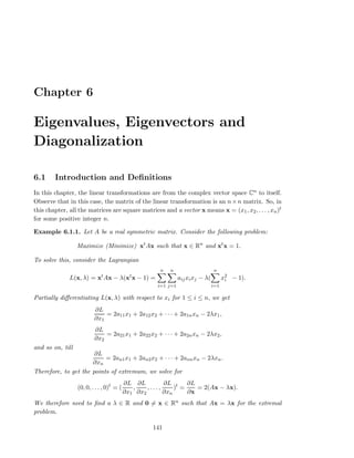
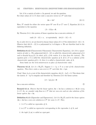
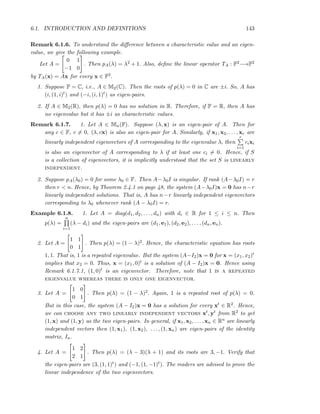
![144 CHAPTER 6. EIGENVALUES, EIGENVECTORS AND DIAGONALIZATION
5. Let A =
1 −1
1 1
. Then p(λ) = λ2 − 2λ + 2 and its roots are 1 + i, 1 − i. Hence, over
R, the matrix A has no eigenvalue. Over C, the reader is required to show that the
eigen-pairs are (1 + i, (i, 1)t) and (1 − i, (1, i)t).
Exercise 6.1.9. 1. Find the eigenvalues of a triangular matrix.
2. Find eigen-pairs over C, for each of the following matrices:
1 1 + i
1 − i 1
,
i 1 + i
−1 + i i
,
cos θ − sin θ
sin θ cos θ
and
cos θ sin θ
sin θ − cos θ
.
3. Let A and B be similar matrices.
(a) Then prove that A and B have the same set of eigenvalues.
(b) If B = PAP−1 for some invertible matrix P then prove that Px is an eigenvector
of B if and only if x is an eigenvector of A.
4. Let A = (aij) be an n × n matrix. Suppose that for all i, 1 ≤ i ≤ n,
n
j=1
aij = a.
Then prove that a is an eigenvalue of A. What is the corresponding eigenvector?
5. Prove that the matrices A and At have the same set of eigenvalues. Construct a 2×2
matrix A such that the eigenvectors of A and At are different.
6. Let A be a matrix such that A2 = A (A is called an idempotent matrix). Then prove
that its eigenvalues are either 0 or 1 or both.
7. Let A be a matrix such that Ak = 0 (A is called a nilpotent matrix) for some positive
integer k ≥ 1. Then prove that its eigenvalues are all 0.
8. Compute the eigen-pairs of the matrices
2 1
−1 0
and
2 i
i 0
.
Theorem 6.1.10. Let A = [aij] be an n × n matrix with eigenvalues λ1, λ2, . . . , λn, not
necessarily distinct. Then det(A) =
n
i=1
λi and tr(A) =
n
i=1
aii =
n
i=1
λi.
Proof. Since λ1, λ2, . . . , λn are the n eigenvalues of A, by definition,
det(A − λIn) = p(λ) = (−1)n
(λ − λ1)(λ − λ2) · · · (λ − λn). (6.1.2)
(6.1.2) is an identity in λ as polynomials. Therefore, by substituting λ = 0 in (6.1.2), we
get
det(A) = (−1)n
(−1)n
n
i=1
λi =
n
i=1
λi.](https://image.slidesharecdn.com/booklinear-160914134339/85/Book-linear-144-320.jpg)
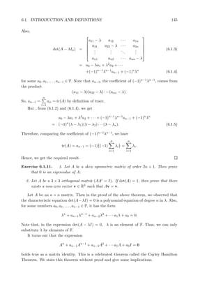
![146 CHAPTER 6. EIGENVALUES, EIGENVECTORS AND DIAGONALIZATION
Theorem 6.1.12 (Cayley Hamilton Theorem). Let A be a square matrix of order n. Then
A satisfies its characteristic equation. That is,
An
+ an−1An−1
+ an−2A2
+ · · · a1A + a0I = 0
holds true as a matrix identity.
Some of the implications of Cayley Hamilton Theorem are as follows.
Remark 6.1.13. 1. Let A =
0 1
0 0
. Then its characteristic polynomial is p(λ) =
λ2. Also, for the function, f(x) = x, f(0) = 0, and f(A) = A = 0. This shows that
the condition f(λ) = 0 for each eigenvalue λ of A does not imply that f(A) = 0.
2. let A be a square matrix of order n with characteristic polynomial p(λ) = λn +
an−1λn−1 + an−2λ2 + · · · a1λ + a0.
(a) Then for any positive integer ℓ, we can use the division algorithm to find numbers
α0, α1, . . . , αn−1 and a polynomial f(λ) such that
λℓ
= f(λ) λn
+ an−1λn−1
+ an−2λ2
+ · · · a1λ + a0
+α0 + λα1 + · · · + λn−1
αn−1.
Hence, by the Cayley Hamilton Theorem,
Aℓ
= α0I + α1A + · · · + αn−1An−1
.
That is, we just need to compute the powers of A till n − 1.
In the language of graph theory, it says the following:
“Let G be a graph on n vertices. Suppose there is no path of length n − 1 or less from
a vertex v to a vertex u of G. Then there is no path from v to u of any length. That is,
the graph G is disconnected and v and u are in different components.”
(b) If A is non-singular then an = det(A) = 0 and hence
A−1
=
−1
an
[An−1
+ an−1An−2
+ · · · + a1I].
This matrix identity can be used to calculate the inverse.
Note that the vector A−1
(as an element of the vector space of all n × n matrices) is a
linear combination of the vectors I, A, . . . , An−1
.
Exercise 6.1.14. Find inverse of the following matrices by using the Cayley Hamilton
Theorem
i)
2 3 4
5 6 7
1 1 2
ii)
−1 −1 1
1 −1 1
0 1 1
iii)
1 −2 −1
−2 1 −1
0 −1 2
.
Theorem 6.1.15. If λ1, λ2, . . . , λk are distinct eigenvalues of a matrix A with correspond-
ing eigenvectors x1, x2, . . . , xk, then the set {x1, x2, . . . , xk} is linearly independent.](https://image.slidesharecdn.com/booklinear-160914134339/85/Book-linear-146-320.jpg)
![6.1. INTRODUCTION AND DEFINITIONS 147
Proof. The proof is by induction on the number m of eigenvalues. The result is obviously
true if m = 1 as the corresponding eigenvector is non-zero and we know that any set
containing exactly one non-zero vector is linearly independent.
Let the result be true for m, 1 ≤ m < k. We prove the result for m + 1. We consider
the equation
c1x1 + c2x2 + · · · + cm+1xm+1 = 0 (6.1.6)
for the unknowns c1, c2, . . . , cm+1. We have
0 = A0 = A(c1x1 + c2x2 + · · · + cm+1xm+1)
= c1Ax1 + c2Ax2 + · · · + cm+1Axm+1
= c1λ1x1 + c2λ2x2 + · · · + cm+1λm+1xm+1. (6.1.7)
From Equations (6.1.6) and (6.1.7), we get
c2(λ2 − λ1)x2 + c3(λ3 − λ1)x3 + · · · + cm+1(λm+1 − λ1)xm+1 = 0.
This is an equation in m eigenvectors. So, by the induction hypothesis, we have
ci(λi − λ1) = 0 for 2 ≤ i ≤ m + 1.
But the eigenvalues are distinct implies λi − λ1 = 0 for 2 ≤ i ≤ m + 1. We therefore get
ci = 0 for 2 ≤ i ≤ m + 1. Also, x1 = 0 and therefore (6.1.6) gives c1 = 0.
Thus, we have the required result.
We are thus lead to the following important corollary.
Corollary 6.1.16. The eigenvectors corresponding to distinct eigenvalues are linearly in-
dependent.
Exercise 6.1.17. 1. Let A, B ∈ Mn(R). Prove that
(a) if λ is an eigenvalue of A then λk is an eigenvalue of Ak for all k ∈ Z+.
(b) if A is invertible and λ is an eigenvalue of A then
1
λ
is an eigenvalue of A−1.
(c) if A is nonsingular then BA−1 and A−1B have the same set of eigenvalues.
(d) AB and BA have the same non-zero eigenvalues.
In each case, what can you say about the eigenvectors?
2. Let A ∈ Mn(R) be an invertible matrix and let xt, yt ∈ Rn with x = 0 and ytA−1x =
0. Define B = xytA−1. Then prove that
(a) λ0 = ytA−1x is an eigenvalue of B of multiplicity 1.
(b) 0 is an eigenvalue of B of multiplicity n − 1 [Hint: Use Exercise 6.1.17.1d].
(c) 1 + αλ0 is an eigenvalue of I + αB of multiplicity 1, for any α ∈ R, α = 0.
(d) 1 is an eigenvalue of I + αB of multiplicity n − 1, for any α ∈ R.](https://image.slidesharecdn.com/booklinear-160914134339/85/Book-linear-147-320.jpg)
![148 CHAPTER 6. EIGENVALUES, EIGENVECTORS AND DIAGONALIZATION
(e) det(A + αxyt) equals (1 + αλ0) det(A) for any α ∈ R. This result is known as
the Shermon-Morrison formula for determinant.
3. Let A, B ∈ M2(R) such that det(A) = det(B) and tr(A) = tr(B).
(a) Do A and B have the same set of eigenvalues?
(b) Give examples to show that the matrices A and B need not be similar.
4. Let A, B ∈ Mn(R). Also, let (λ1, u) be an eigen-pair for A and (λ2, v) be an eigen-
pair for B.
(a) If u = αv for some α ∈ R then (λ1 + λ2, u) is an eigen-pair for A + B.
(b) Give an example to show that if u and v are linearly independent then λ1 + λ2
need not be an eigenvalue of A + B.
5. Let A ∈ Mn(R) be an invertible matrix with eigen-pairs (λ1, u1), (λ2, u2), . . . , (λn, un).
Then prove that B = {u1, u2, . . . , un} forms a basis of Rn(R). If [b]B = (c1, c2, . . . , cn)t
then the system Ax = b has the unique solution
x =
c1
λ1
u1 +
c2
λ2
u2 + · · · +
cn
λn
un.
6.2 Diagonalization
Let A ∈ Mn(F) and let TA : Fn−→Fn be the corresponding linear operator. In this section,
we ask the question “does there exist a basis B of Fn such that TA[B, B], the matrix of the
linear operator TA with respect to the ordered basis B, is a diagonal matrix.” it will be
shown that for a certain class of matrices, the answer to the above question is in affirmative.
To start with, we have the following definition.
Definition 6.2.1 (Matrix Digitalization). A matrix A is said to be diagonalizable if there
exists a non-singular matrix P such that P−1AP is a diagonal matrix.
Remark 6.2.2. Let A ∈ Mn(F) be a diagonalizable matrix with eigenvalues λ1, λ2, . . . , λn.
By definition, A is similar to a diagonal matrix D = diag(λ1, λ2, . . . , λn) as similar matrices
have the same set of eigenvalues and the eigenvalues of a diagonal matrix are its diagonal
entries.
Example 6.2.3. Let A =
0 1
−1 0
. Then we have the following:
1. Let V = R2. Then A has no real eigenvalue (see Example 6.1.7 and hence A doesn’t
have eigenvectors that are vectors in R2. Hence, there does not exist any non-singular
2 × 2 real matrix P such that P−1AP is a diagonal matrix.](https://image.slidesharecdn.com/booklinear-160914134339/85/Book-linear-148-320.jpg)
![6.2. DIAGONALIZATION 149
2. In case, V = C2(C), the two complex eigenvalues of A are −i, i and the corresponding
eigenvectors are (i, 1)t and (−i, 1)t, respectively. Also, (i, 1)t and (−i, 1)t can be taken
as a basis of C2(C). Define U = 1√
2
i −i
1 1
. Then
U∗
AU =
−i 0
0 i
.
Theorem 6.2.4. Let A ∈ Mn(R). Then A is diagonalizable if and only if A has n linearly
independent eigenvectors.
Proof. Let A be diagonalizable. Then there exist matrices P and D such that
P−1
AP = D = diag(λ1, λ2, . . . , λn).
Or equivalently, AP = PD. Let P = [u1, u2, . . . , un]. Then AP = PD implies that
Aui = diui for 1 ≤ i ≤ n.
Since ui’s are the columns of a non-singular matrix P, using Corollary 4.3.10, they form
a linearly independent set. Thus, we have shown that if A is diagonalizable then A has n
linearly independent eigenvectors.
Conversely, suppose A has n linearly independent eigenvectors ui, 1 ≤ i ≤ n with
eigenvalues λi. Then Aui = λiui. Let P = [u1, u2, . . . , un]. Since u1, u2, . . . , un are linearly
independent, by Corollary 4.3.10, P is non-singular. Also,
AP = [Au1, Au2, . . . , Aun] = [λ1u1, λ2u2, . . . , λnun]
= [u1, u2, . . . , un]
λ1 0 0
0 λ2 0
...
...
...
0 0 λn
= PD.
Therefore, the matrix A is diagonalizable.
Corollary 6.2.5. If the eigenvalues of a A ∈ Mn(R) are distinct then A is diagonalizable.
Proof. As A ∈ Mn(R), it has n eigenvalues. Since all the eigenvalues of A are distinct, by
Corollary 6.1.16, the n eigenvectors are linearly independent. Hence, by Theorem 6.2.4, A
is diagonalizable.
Corollary 6.2.6. Let λ1, λ2, . . . , λk be distinct eigenvalues of A ∈ Mn(R) and let p(λ) be
its characteristic polynomial. Suppose that for each i, 1 ≤ i ≤ k, (x − λi)mi divides p(λ)
but (x − λi)mi+1 does not divides p(λ) for some positive integers mi. Then prove that A is
diagonalizable if and only if dim ker(A − λiI) = mi for each i, 1 ≤ i ≤ k. Or equivalently
A is diagonalizable if and only if rank(A − λiI) = n − mi for each i, 1 ≤ i ≤ k.](https://image.slidesharecdn.com/booklinear-160914134339/85/Book-linear-149-320.jpg)
![150 CHAPTER 6. EIGENVALUES, EIGENVECTORS AND DIAGONALIZATION
Proof. As A is diagonalizable, by Theorem 6.2.4, A has n linearly independent eigenvalues.
Also, by assumption,
k
i=1
mi = n as deg(p(λ)) = n. Hence, for each eigenvalue λi, 1 ≤ i ≤ k,
A has exactly mi linearly independent eigenvectors. Thus, for each i, 1 ≤ i ≤ k, the
homogeneous linear system (A − λiI)x = 0 has exactly mi linearly independent vectors in
its solution set. Therefore, dim ker(A − λiI) ≥ mi. Indeed dim ker(A − λiI) = mi for
1 ≤ i ≤ k follows from a simple counting argument.
Now suppose that for each i, 1 ≤ i ≤ k, dim ker(A−λiI) = mi. Then for each i, 1 ≤
i ≤ k, we can choose mi linearly independent eigenvectors. Also by Corollary 6.1.16, the
eigenvectors corresponding to distinct eigenvalues are linearly independent. Hence A has
n =
k
i=1
mi linearly independent eigenvectors. Hence by Theorem 6.2.4, A is diagonalizable.
Example 6.2.7. 1. Let A =
2 1 1
1 2 1
0 −1 1
. Then pA(λ) = (2 − λ)2(1 − λ). Hence,
the eigenvalues of A are 1, 2, 2. Verify that 1, (1, 0, −1)t and ( 2, (1, 1, −1)t are the
only eigen-pairs. That is, the matrix A has exactly one eigenvector corresponding to
the repeated eigenvalue 2. Hence, by Theorem 6.2.4, A is not diagonalizable.
2. Let A =
2 1 1
1 2 1
1 1 2
. Then pA(λ) = (4−λ)(1−λ)2. Hence, A has eigenvalues 1, 1, 4.
Verify that u1 = (1, −1, 0)t and u2 = (1, 0, −1)t are eigenvectors corresponding to 1
and u3 = (1, 1, 1)t is an eigenvector corresponding to the eigenvalue 4. As u1, u2, u3
are linearly independent, by Theorem 6.2.4, A is diagonalizable.
Note that the vectors u1 and u2 (corresponding to the eigenvalue 1) are not orthogo-
nal. So, in place of u1, u2, we will take the orthogonal vectors u2 and w = 2u1 − u2
as eigenvectors. Now define U = [ 1√
3
u3, 1√
2
u2, 1√
6
w] =
1√
3
1√
2
1√
6
1√
3
0 −2√
6
1√
3
− 1√
2
1√
6
. Then U
is an orthogonal matrix and U∗AU = diag(4, 1, 1).
Observe that A is a symmetric matrix. In this case, we chose our eigenvectors to be
mutually orthogonal. This result is true for any real symmetric matrix A. This result
will be proved later.
Exercise 6.2.8. 1. Are the matrices A =
cos θ sin θ
− sin θ cos θ
and B =
cos θ sin θ
sin θ − cos θ
for some θ, 0 ≤ θ ≤ 2π, diagonalizable?
2. Find the eigen-pairs of A = [aij]n×n, where aij = a if i = j and b, otherwise.
3. Let A ∈ Mn(R) and B ∈ Mm(R). Suppose C =
A 0
0 B
. Then prove that C is
diagonalizable if and only if both A and B are diagonalizable.](https://image.slidesharecdn.com/booklinear-160914134339/85/Book-linear-150-320.jpg)
![6.3. DIAGONALIZABLE MATRICES 151
4. Let T : R5 −→ R5 be a linear operator with rank (T − I) = 3 and
N(T) = {(x1, x2, x3, x4, x5) ∈ R5
| x1 + x4 + x5 = 0, x2 + x3 = 0}.
(a) Determine the eigenvalues of T?
(b) Find the number of linearly independent eigenvectors corresponding to each
eigenvalue?
(c) Is T diagonalizable? Justify your answer.
5. Let A be a non-zero square matrix such that A2 = 0. Prove that A cannot be diago-
nalized. [Hint: Use Remark 6.2.2.]
6. Are the following matrices diagonalizable?
i)
1 3 2 1
0 2 3 1
0 0 −1 1
0 0 0 4
, ii)
1 0 −1
0 0 1
0 2 0
, iii)
1 −3 3
0 −5 6
0 −3 4
and iv)
2 i
i 0
.
6.3 Diagonalizable Matrices
In this section, we will look at some special classes of square matrices that are diagonal-
izable. Recall that for a matrix A = [aij], A∗ = [aji] = At = A
t
, is called the conjugate
transpose of A. We also recall the following definitions.
Definition 6.3.1 (Special Matrices). 1. A matrix A ∈ Mn(C) is called
(a) a Hermitian matrix if A∗ = A.
(b) a unitary matrix if A A∗ = A∗A = In.
(c) a skew-Hermitian matrix if A∗ = −A.
(d) a normal matrix if A∗A = AA∗.
2. A matrix A ∈ Mn(R) is called
(a) a symmetric matrix if At = A.
(b) an orthogonal matrix if A At = AtA = In.
(c) a skew-symmetric matrix if At = −A.
Note that a symmetric matrix is always Hermitian, a skew-symmetric matrix is always
skew-Hermitian and an orthogonal matrix is always unitary. Each of these matrices are
normal. If A is a unitary matrix then A∗ = A−1.
Example 6.3.2. 1. Let B =
i 1
−1 i
. Then B is skew-Hermitian.
2. Let A = 1√
2
1 i
i 1
and B =
1 1
−1 1
. Then A is a unitary matrix and B is a
normal matrix. Note that
√
2A is also a normal matrix.](https://image.slidesharecdn.com/booklinear-160914134339/85/Book-linear-151-320.jpg)
![152 CHAPTER 6. EIGENVALUES, EIGENVECTORS AND DIAGONALIZATION
Definition 6.3.3 (Unitary Equivalence). Let A, B ∈ Mn(C). They are called unitarily
equivalent if there exists a unitary matrix U such that A = U∗BU. As U is a unitary
matrix, U∗ = U−1. Hence, A is also unitarily similar to B.
Exercise 6.3.4. 1. Let A be a square matrix such that UAU∗ is a diagonal matrix for
some unitary matrix U. Prove that A is a normal matrix.
2. Let A ∈ Mn(C). Then A = 1
2(A+A∗)+ 1
2(A−A∗), where 1
2(A+A∗) is the Hermitian
part of A and 1
2(A − A∗) is the skew-Hermitian part of A. Recall that a similar result
was given in Exercise 1.3.3.1.
3. Let A ∈ Mn(C). Prove that A − A∗ is always skew-Hermitian.
4. Every square matrix can be uniquely expressed as A = S + iT, where both S and T
are Hermitian matrices.
5. Does there exist a unitary matrix U such that U−1AU = B where
A =
1 1 4
0 2 2
0 0 3
and B =
2 −1 3
√
2
0 1
√
2
0 0 3
.
Theorem 6.3.5. Let A ∈ Mn(C) be a Hermitian matrix. Then
1. the eigenvalues, λi, 1 ≤ i ≤ n, of A are real.
2. A is unitarily diagonalizable. That is, there exists a unitary matrix U such that
U∗AU = D; where D = diag(λ1, . . . , λn). In other words, the eigenvectors of A
form an orthonormal basis of Cn.
Proof. For the proof of Part 1, let (λ, x) be an eigen-pair. Then Ax = λx and A∗ = A
implies that x∗A = x∗A∗ = (Ax)∗ = (λx)∗ = λx∗. Hence,
λx∗
x = x∗
(λx) = x∗
(Ax) = (x∗
A)x = (λx∗
)x = λx∗
x.
As x is an eigenvector, x = 0 and therefore x 2 = x∗x = 0. Thus λ = λ. That is, λ is a
real number.
For the proof of Part 2, we use induction on n, the size of the matrix. The result is
clearly true for n = 1. Let the result be true for n = k − 1. we need to prove the result for
n = k.
Let (λ1, x) be an eigen-pair of a k × k matrix A with x = 1. Then by Part 1,
λ1 ∈ R. As {x} is a linearly independent set, by Theorem 3.3.11 and the Gram-Schmidt
Orthogonalization process, we get an orthonormal basis {x, u2, . . . , uk} of Ck. Let U1 =
[x, u2, . . . , uk] (the vectors x, u2, . . . , uk are columns of the matrix U1). Then U1 is a
unitary matrix. In particular, u∗
i x = 0, for 2 ≤ i ≤ k. Therefore, for 2 ≤ i ≤ k,
x∗
(Aui) = (Aui)∗
x = (u∗
i A∗
)x = u∗
i (A∗
x) = u∗
i (Ax) = u∗
i (λ1x) = λ1(u∗
i x) = 0 and](https://image.slidesharecdn.com/booklinear-160914134339/85/Book-linear-152-320.jpg)
![6.3. DIAGONALIZABLE MATRICES 153
U∗
1 AU1 = U∗
1 [Ax, Au2, · · · , Auk] =
x∗
u∗
2
...
u∗
k
[λ1x, Au2, · · · , Auk]
=
λ1x∗x · · · x∗Auk
u∗
2(λ1x) · · · u∗
2(Auk)
...
...
...
u∗
k(λ1x) · · · u∗
k(Auk)
=
λ1 0
0
... B
0
,
where B is a (k − 1) × (k − 1) matrix. As (U∗
1 AU1)∗ = U∗
1 AU1 and λ1 ∈ R, the matrix B is
also Hermitian. Therefore, by induction hypothesis there exists a (k − 1) × (k − 1) unitary
matrix U2 such that U∗
2 BU2 = D2 = diag(λ2, . . . , λk), where λi ∈ R, for 2 ≤ i ≤ k are the
eigenvalues of B. Define U = U1
1 0
0 U2
. Then U is a unitary matrix and
U∗
AU = U1
1 0
0 U2
∗
A U1
1 0
0 U2
=
1 0
0 U∗
2
U∗
1 A U1
1 0
0 U2
=
1 0
0 U∗
2
U∗
1 AU1
1 0
0 U2
=
1 0
0 U∗
2
λ1 0
0 B
1 0
0 U2
=
λ1 0
0 U∗
2 BU2
=
λ1 0
0 D2
.
Observe that λ2, . . . , λn are also the eigenvalues of A. Thus, U∗AU is a diagonal matrix
with diagonal entries λ1, λ2, . . . , λk, the eigenvalues of A. Hence, the result follows.
Corollary 6.3.6. Let A ∈ Mn(R) be a symmetric matrix. Then
1. the eigenvalues of A are all real,
2. the eigenvectors can be chosen to have real entries and
3. the eigenvectors also form an orthonormal basis of Rn.
Proof. As A is symmetric, A is also a Hermitian matrix. Hence, by Theorem 6.3.5, the
eigenvalues of A are all real. Let (λ, x) be an eigen-pair of A. Suppose xt ∈ Cn. Then
there exist yt, zt ∈ Rn such that x = y + iz. So,
Ax = λx =⇒ A(y + iz) = λ(y + iz).
Comparing the real and imaginary parts, we get Ay = λy and Az = λz. Thus, we can
choose the eigenvectors to have real entries.
The readers are advised to prove the orthonormality of the eigenvectors (see the proof
of Theorem 6.3.5).](https://image.slidesharecdn.com/booklinear-160914134339/85/Book-linear-153-320.jpg)
![154 CHAPTER 6. EIGENVALUES, EIGENVECTORS AND DIAGONALIZATION
Exercise 6.3.7. 1. Let A be a skew-Hermitian matrix. Then the eigenvalues of A are
either zero or purely imaginary. Also, the eigenvectors corresponding to distinct
eigenvalues are mutually orthogonal. [Hint: Carefully see the proof of Theorem 6.3.5.]
2. Let A be a normal matrix with (λ, x) as an eigen-pair. Then
(a) (A∗)kx for k ∈ Z+ is also an eigenvector corresponding to λ.
(b) (λ, x) is an eigen-pair for A∗. [Hint: Verify A∗x − λx 2 = Ax − λx 2.]
3. Let A be an n × n unitary matrix. Then
(a) the rows of A form an orthonormal basis of Cn.
(b) the columns of A form an orthonormal basis of Cn.
(c) for any two vectors x, y ∈ Cn×1, Ax, Ay = x, y .
(d) for any vector x ∈ Cn×1, Ax = x .
(e) |λ| = 1 for any eigenvalue λ of A.
(f) the eigenvectors x, y corresponding to distinct eigenvalues λ and µ satisfy x, y =
0. That is, if (λ, x) and (µ, y) are eigen-pairs with λ = µ, then x and y are mu-
tually orthogonal.
4. Show that the matrices A =
4 4
0 4
and B =
10 9
−4 −2
are similar. Is it possible to
find a unitary matrix U such that A = U∗BU?
5. Let A be a 2 × 2 orthogonal matrix. Then prove the following:
(a) if det(A) = 1, then A =
cos θ − sin θ
sin θ cos θ
for some θ, 0 ≤ θ < 2π. That is, A
counterclockwise rotates every point in R2 by an angle θ.
(b) if det A = −1, then A =
cos θ sin θ
sin θ − cos θ
for some θ, 0 ≤ θ < 2π. That is, A
reflects every point in R2 about a line passing through origin. Determine this
line. Or equivalently, there exists a non-singular matrix P such that P−1AP =
1 0
0 −1
.
6. Let A be a 3 × 3 orthogonal matrix. Then prove the following:
(a) if det(A) = 1, then A is a rotation about a fixed axis, in the sense that A
has an eigen-pair (1, x) such that the restriction of A to the plane x⊥ is a two
dimensional rotation in x⊥.
(b) if det A = −1, then A corresponds to a reflection through a plane P, followed by
a rotation about the line through origin that is orthogonal to P.](https://image.slidesharecdn.com/booklinear-160914134339/85/Book-linear-154-320.jpg)
![6.3. DIAGONALIZABLE MATRICES 155
7. Let A =
2 1 1
1 2 1
1 1 2
. Find a non-singular matrix P such that P−1AP = diag (4, 1, 1).
Use this to compute A301.
8. Let A be a Hermitian matrix. Then prove that rank(A) equals the number of non-zero
eigenvalues of A.
Remark 6.3.8. Let A and B be the 2 × 2 matrices in Exercise 6.3.7.4. Then A and B
were similar matrices but they were not unitarily equivalent. In numerical calculations,
unitary transformations are preferred as compared to similarity transformations due to the
following main reasons:
1. Exercise 6.3.7.3d implies that an orthonormal change of basis does not alter the sum
of squares of the absolute values of the entries. This need not be true under a non-
singularity change of basis.
2. For a unitary matrix U, U−1 = U∗ and hence unitary equivalence is computationally
simpler.
3. Also there is no round-off error in the operation of “conjugate transpose”.
We next prove the Schur’s Lemma and use it to show that normal matrices are unitarily
diagonalizable. The proof is similar to the proof of Theorem 6.3.5. We give it again so
that the readers have a better understanding of unitary transformations.
Lemma 6.3.9. (Schur’s Lemma) Let A ∈ Mn(C). Then A is unitarily similar to an upper
triangular matrix.
Proof. We will prove the result by induction on n. The result is clearly true for n = 1. Let
the result be true for n = k − 1. we need to prove the result for n = k.
Let (λ1, x) be an eigen-pair of a k × k matrix A with x = 1. Let us extend the set
{x}, a linearly independent set, to form an orthonormal basis {x, u2, u3, . . . , uk} (using
Gram-Schmidt Orthogonalization) of Ck. Then U1 = [x u2 · · · uk] is a unitary matrix and
U∗
1 AU1 = U∗
1 [Ax Au2 · · · Auk] =
x∗
u∗
2
...
u∗
k
[λ1x Au2 · · · Auk] =
λ1 ∗
0
... B
0
,
where B is a (k−1)×(k−1) matrix. By induction hypothesis there exists a (k−1)×(k−1)
unitary matrix U2 such that U∗
2 BU2 is an upper triangular matrix with diagonal entries
λ2, . . . , λk, the eigenvalues of B. Define U = U1
1 0
0 U2
. Then check that U is a unitary
matrix and U∗AU is an upper triangular matrix with diagonal entries λ1, λ2, . . . , λk, the
eigenvalues of the matrix A. Hence, the result follows.](https://image.slidesharecdn.com/booklinear-160914134339/85/Book-linear-155-320.jpg)
![156 CHAPTER 6. EIGENVALUES, EIGENVECTORS AND DIAGONALIZATION
In Lemma 6.3.9, it can be observed that whenever A is a normal matrix then the matrix
B is also a normal matrix. It is also known that if T is an upper triangular matrix that
satisfies TT∗ = T∗T then T is a diagonal matrix (see Exercise 16). Thus, it follows that
normal matrices are diagonalizable. We state it as a remark.
Remark 6.3.10 (The Spectral Theorem for Normal Matrices). Let A be an n × n normal
matrix. Then there exists an orthonormal basis {x1, x2, . . . , xn} of Cn(C) such that Axi =
λixi for 1 ≤ i ≤ n. In particular, if U − [x1, x2, . . . , xn] then U∗AU is a diagonal matrix.
Exercise 6.3.11. 1. Let A ∈ Mn(R) be an invertible matrix. Prove that AAt = PDPt,
where P is an orthogonal and D is a diagonal matrix with positive diagonal entries.
2. Let A =
1 1 1
0 2 1
0 0 3
, B =
2 −1
√
2
0 1 0
0 0 3
and U = 1√
2
1 1 0
1 −1 0
0 0
√
2
. Prove that A
and B are unitarily equivalent via the unitary matrix U. Hence, conclude that the
upper triangular matrix obtained in the ”Schur’s Lemma” need not be unique.
3. Prove Remark 6.3.10.
4. Let A be a normal matrix. If all the eigenvalues of A are 0 then prove that A = 0.
What happens if all the eigenvalues of A are 1?
5. Let A be an n × n matrix. Prove that if A is
(a) Hermitian and xAx∗ = 0 for all x ∈ Cn then A = 0.
(b) a real, symmetric matrix and xAxt = 0 for all x ∈ Rn then A = 0.
Do these results hold for arbitrary matrices?
We end this chapter with an application of the theory of diagonalization to the study
of conic sections in analytic geometry and the study of maxima and minima in analysis.
6.4 Sylvester’s Law of Inertia and Applications
Definition 6.4.1 (Bilinear Form). Let A be an n × n real symmetric matrix. A bilinear
form in x = (x1, x2, . . . , xn)t, y = (y1, y2, . . . , yn)t is an expression of the type
Q(x, y) = yt
Ax =
n
i,j=1
aijxiyj.
Definition 6.4.2 (Sesquilinear Form). Let A be an n×n Hermitian matrix. A sesquilinear
form in x = (x1, x2, . . . , xn)∗, y = (y1, y2, . . . , yn)∗ is given by
H(x, y) = y∗
Ax =
n
i,j=1
aijxiyj.](https://image.slidesharecdn.com/booklinear-160914134339/85/Book-linear-156-320.jpg)
![6.4. SYLVESTER’S LAW OF INERTIA AND APPLICATIONS 157
Observe that if A = In then the bilinear (sesquilinear) form reduces to the standard
real (complex) inner product. Also, it can be easily seen that H(x, y) is ‘linear’ in x, the
first component and ‘conjugate linear’ in y, the second component. The expression Q(x, x)
is called the quadratic form and H(x, x) the Hermitian form. We generally write Q(x) and
H(x) in place of Q(x, x) and H(x, x), respectively. It can be easily shown that for any
choice of x, the Hermitian form H(x) is a real number. Hence, for any real number α, the
equation H(x) = α, represents a conic in Cn.
Example 6.4.3. Let A =
1 2 − i
2 + i 2
. Then A∗ = A and for x = (x1, x2)∗,
H(x) = x∗
Ax = (x1, x2)
1 2 − i
2 + i 2
x1
x2
= x1x1 + 2x2x2 + (2 − i)x1x2 + (2 + i)x2x1
= |x1|2
+ 2|x2|2
+ 2Re[(2 − i)x1x2]
where ‘Re’ denotes the real part of a complex number. This shows that for every choice of
x the Hermitian form is always real. Why?
The main idea of this section is to express H(x) as sum of squares and hence determine
the possible values that it can take. Note that if we replace x by cx, where c is any complex
number, then H(x) simply gets multiplied by |c|2 and hence one needs to study only those
x for which x = 1, i.e., x is a normalized vector.
Let A∗ = A ∈ Mn(C). Then by Theorem 6.3.5, the eigenvalues λi, 1 ≤ i ≤ n, of A
are real and there exists a unitary matrix U such that U∗AU = D ≡ diag(λ1, λ2, . . . , λn).
Now define, z = (z1, z2, . . . , zn)∗ = U∗x. Then z = 1, x = Uz and
H(x) = z∗
U∗
AUz = z∗
Dz =
n
i=1
λi|zi|2
=
p
i=1
|λi| zi
2
−
r
i=p+1
|λi| zi
2
. (6.4.1)
Thus, the possible values of H(x) depend only on the eigenvalues of A. Since U is an invert-
ible matrix, the components zi’s of z = U∗x are commonly known as linearly independent
linear forms. Also, note that in Equation (6.4.1), the number p (respectively r − p) seems
to be related to the number of eigenvalues of A that are positive (respectively negative).
This is indeed true. That is, in any expression of H(x) as a sum of n absolute squares of
linearly independent linear forms, the number p (respectively r − p) gives the number of
positive (respectively negative) eigenvalues of A. This is stated as the next lemma and it
popularly known as the ‘Sylvester’s law of inertia’.
Lemma 6.4.4. Let A ∈ Mn(C) be a Hermitian matrix and let x = (x1, x2, . . . , xn)∗. Then
every Hermitian form H(x) = x∗Ax, in n variables can be written as
H(x) = |y1|2
+ |y2|2
+ · · · + |yp|2
− |yp+1|2
− · · · − |yr|2
where y1, y2, . . . , yr are linearly independent linear forms in x1, x2, . . . , xn, and the integers
p and r satisfying 0 ≤ p ≤ r ≤ n, depend only on A.](https://image.slidesharecdn.com/booklinear-160914134339/85/Book-linear-157-320.jpg)
![158 CHAPTER 6. EIGENVALUES, EIGENVECTORS AND DIAGONALIZATION
Proof. From Equation (6.4.1) it is easily seen that H(x) has the required form. We only
need to show that p and r are uniquely determined by A. Hence, let us assume on the
contrary that there exist positive integers p, q, r, s with p > q such that
H(x) = |y1|2
+ |y2|2
+ · · · + |yp|2
− |yp+1|2
− · · · − |yr|2
= |z1|2
+ |z2|2
+ · · · + |zq|2
− |zq+1|2
− · · · − |zs|2
,
where y = (y1, y2, . . . , yn)∗ = Mx and z = (z1, z2, . . . , zn)∗ = Nx for some invertible
matrices M and N. Hence, z = By for some invertible matrix B. Let us write Y1 =
(y1, . . . , yp)∗, Z1 = (z1, . . . , zq)∗ and B =
B1 B2
B3 B4
, where B1 is a q × p matrix. As p > q,
the homogeneous linear system B1Y1 = 0 has a non-zero solution. Let ˜Y1 = ( ˜y1, . . . , ˜yp)∗
be a non-zero solution and let ˜y∗ = ( ˜Y1
∗
, 0∗). Then
H(˜y) = | ˜y1|2
+ | ˜y2|2
+ · · · + | ˜yp|2
= −(|zq+1|2
+ · · · + |zs|2
).
Now, this can hold only if ˜y1 = ˜y2 = · · · = ˜yp = 0, which gives a contradiction. Hence
p = q. Similarly, the case r > s can be resolved. Thus, the proof of the lemma is over.
Remark 6.4.5. The integer r is the rank of the matrix A and the number r − 2p is
sometimes called the inertial degree of A.
We complete this chapter by understanding the graph of
ax2
+ 2hxy + by2
+ 2fx + 2gy + c = 0
for a, b, c, f, g, h ∈ R. We first look at the following example.
Example 6.4.6. Sketch the graph of 3x2 + 4xy + 3y2 = 5.
Solution: Note that 3x2 + 4xy + 3y2 = [x, y]
3 2
2 3
x
y
and the eigen-pairs of the
matrix
3 2
2 3
are (5, (1, 1)t), (1, (1, −1)t). Thus,
3 2
2 3
=
1√
2
1√
2
1√
2
− 1√
2
5 0
0 1
1√
2
1√
2
1√
2
− 1√
2
.
Now, let u = x+y√
2
and v = x−y√
2
. Then
3x2
+ 4xy + 3y2
= [x, y]
3 2
2 3
x
y
= [x, y]
1√
2
1√
2
1√
2
− 1√
2
5 0
0 1
1√
2
1√
2
1√
2
− 1√
2
x
y
= u, v
5 0
0 1
u
v
= 5u2
+ v2
.](https://image.slidesharecdn.com/booklinear-160914134339/85/Book-linear-158-320.jpg)
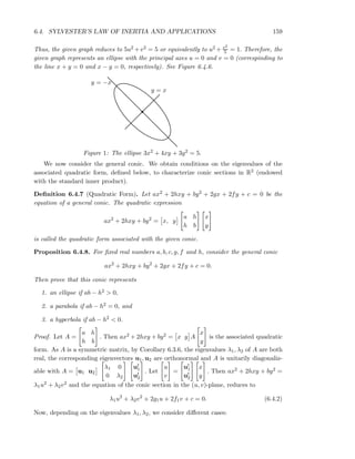
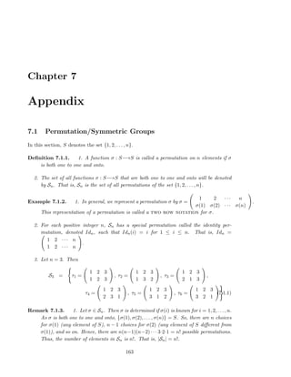
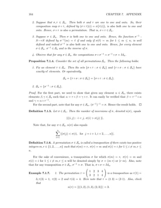
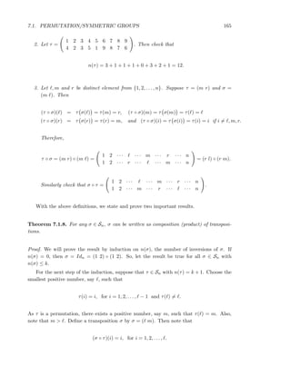
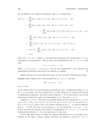
![168 CHAPTER 7. APPENDIX
2. Using Remark 7.1.12, sgn(σ◦τ) = sgn(σ)·sgn(τ) for any two permutations σ, τ ∈ Sn.
We are now ready to define determinant of a square matrix A.
Definition 7.1.15. Let A = [aij] be an n×n matrix with entries from F. The determinant
of A, denoted det(A), is defined as
det(A) =
σ∈Sn
sgn(σ)a1σ(1)a2σ(2) . . . anσ(n) =
σ∈Sn
sgn(σ)
n
i=1
aiσ(i).
Remark 7.1.16. 1. Observe that det(A) is a scalar quantity. The expression for det(A)
seems complicated at the first glance. But this expression is very helpful in proving
the results related with “properties of determinant”.
2. If A = [aij] is a 3 × 3 matrix, then using (7.1.1),
det(A) =
σ∈Sn
sgn(σ)
3
i=1
aiσ(i)
= sgn(τ1)
3
i=1
aiτ1(i) + sgn(τ2)
3
i=1
aiτ2(i) + sgn(τ3)
3
i=1
aiτ3(i) +
sgn(τ4)
3
i=1
aiτ4(i) + sgn(τ5)
3
i=1
aiτ5(i) + sgn(τ6)
3
i=1
aiτ6(i)
= a11a22a33 − a11a23a32 − a12a21a33 + a12a23a31 + a13a21a32 − a13a22a31.
Observe that this expression for det(A) for a 3 × 3 matrix A is same as that given in
(2.5.1).
7.2 Properties of Determinant
Theorem 7.2.1 (Properties of Determinant). Let A = [aij] be an n × n matrix. Then
1. if B is obtained from A by interchanging two rows, then
det(B) = − det(A).
2. if B is obtained from A by multiplying a row by c then
det(B) = c det(A).
3. if all the elements of one row is 0 then det(A) = 0.
4. if A is a square matrix having two rows equal then det(A) = 0.
5. Let B = [bij] and C = [cij] be two matrices which differ from the matrix A = [aij]
only in the mth row for some m. If cmj = amj + bmj for 1 ≤ j ≤ n then det(C) =
det(A) + det(B).
6. if B is obtained from A by replacing the ℓth row by itself plus k times the mth row,
for ℓ = m then det(B) = det(A).](https://image.slidesharecdn.com/booklinear-160914134339/85/Book-linear-168-320.jpg)
![7.2. PROPERTIES OF DETERMINANT 169
7. if A is a triangular matrix then det(A) = a11a22 · · · ann, the product of the diagonal
elements.
8. If E is an elementary matrix of order n then det(EA) = det(E) det(A).
9. A is invertible if and only if det(A) = 0.
10. If B is an n × n matrix then det(AB) = det(A) det(B).
11. det(A) = det(At), where recall that At is the transpose of the matrix A.
Proof. Proof of Part 1. Suppose B = [bij] is obtained from A = [aij] by the interchange
of the ℓth and mth row. Then bℓj = amj, bmj = aℓj for 1 ≤ j ≤ n and bij = aij for
1 ≤ i = ℓ, m ≤ n, 1 ≤ j ≤ n.
Let τ = (ℓ m) be a transposition. Then by Proposition 7.1.4, Sn = {σ ◦ τ : σ ∈ Sn}.
Hence by the definition of determinant and Example 7.1.14.2, we have
det(B) =
σ∈Sn
sgn(σ)
n
i=1
biσ(i) =
σ◦τ∈Sn
sgn(σ ◦ τ)
n
i=1
bi(σ◦τ)(i)
=
σ◦τ∈Sn
sgn(τ) · sgn(σ) b1(σ◦τ)(1)b2(σ◦τ)(2) · · · bℓ(σ◦τ)(ℓ) · · · bm(σ◦τ)(m) · · · bn(σ◦τ)(n)
= sgn(τ)
σ∈Sn
sgn(σ) b1σ(1) · b2σ(2) · · · bℓσ(m) · · · bmσ(ℓ) · · · bnσ(n)
= −
σ∈Sn
sgn(σ) a1σ(1) · a2σ(2) · · · amσ(m) · · · aℓσ(ℓ) · · · anσ(n) as sgn(τ) = −1
= − det(A).
Proof of Part 2. Suppose that B = [bij] is obtained by multiplying the mth row of A
by c = 0. Then bmj = c amj and bij = aij for 1 ≤ i = m ≤ n, 1 ≤ j ≤ n. Then
det(B) =
σ∈Sn
sgn(σ)b1σ(1)b2σ(2) · · · bmσ(m) · · · bnσ(n)
=
σ∈Sn
sgn(σ)a1σ(1)a2σ(2) · · · camσ(m) · · · anσ(n)
= c
σ∈Sn
sgn(σ)a1σ(1)a2σ(2) · · · amσ(m) · · · anσ(n)
= c det(A).
Proof of Part 3. Note that det(A) =
σ∈Sn
sgn(σ)a1σ(1)a2σ(2) . . . anσ(n). So, each term
in the expression for determinant, contains one entry from each row. Hence, from the
condition that A has a row consisting of all zeros, the value of each term is 0. Thus,
det(A) = 0.
Proof of Part 4. Suppose that the ℓth and mth row of A are equal. Let B be the
matrix obtained from A by interchanging the ℓth and mth rows. Then by the first part,](https://image.slidesharecdn.com/booklinear-160914134339/85/Book-linear-169-320.jpg)
![170 CHAPTER 7. APPENDIX
det(B) = − det(A). But the assumption implies that B = A. Hence, det(B) = det(A). So,
we have det(B) = − det(A) = det(A). Hence, det(A) = 0.
Proof of Part 5. By definition and the given assumption, we have
det(C) =
σ∈Sn
sgn(σ)c1σ(1)c2σ(2) · · · cmσ(m) · · · cnσ(n)
=
σ∈Sn
sgn(σ)c1σ(1)c2σ(2) · · · (bmσ(m) + amσ(m)) · · · cnσ(n)
=
σ∈Sn
sgn(σ)b1σ(1)b2σ(2) · · · bmσ(m) · · · bnσ(n)
+
σ∈Sn
sgn(σ)a1σ(1)a2σ(2) · · · amσ(m) · · · anσ(n)
= det(B) + det(A).
Proof of Part 6. Suppose that B = [bij] is obtained from A by replacing the ℓth row
by itself plus k times the mth row, for ℓ = m. Then bℓj = aℓj + k amj and bij = aij for
1 ≤ i = m ≤ n, 1 ≤ j ≤ n. Then
det(B) =
σ∈Sn
sgn(σ)b1σ(1)b2σ(2) · · · bℓσ(ℓ) · · · bmσ(m) · · · bnσ(n)
=
σ∈Sn
sgn(σ)a1σ(1)a2σ(2) · · · (aℓσ(ℓ) + kamσ(m)) · · · amσ(m) · · · anσ(n)
=
σ∈Sn
sgn(σ)a1σ(1)a2σ(2) · · · aℓσ(ℓ) · · · amσ(m) · · · anσ(n)
+k
σ∈Sn
sgn(σ)a1σ(1)a2σ(2) · · · amσ(m) · · · amσ(m) · · · anσ(n)
=
σ∈Sn
sgn(σ)a1σ(1)a2σ(2) · · · aℓσ(ℓ) · · · amσ(m) · · · anσ(n) use Part 4
= det(A).
Proof of Part 7. First let us assume that A is an upper triangular matrix. Observe
that if σ ∈ Sn is different from the identity permutation then n(σ) ≥ 1. So, for every
σ = Idn ∈ Sn, there exists a positive integer m, 1 ≤ m ≤ n − 1 (depending on σ) such
that m > σ(m). As A is an upper triangular matrix, amσ(m) = 0 for each σ(= Idn) ∈ Sn.
Hence the result follows.
A similar reasoning holds true, in case A is a lower triangular matrix.
Proof of Part 8. Let In be the identity matrix of order n. Then using Part 7, det(In) = 1.
Also, recalling the notations for the elementary matrices given in Remark 2.2.2, we have
det(Eij) = −1, (using Part 1) det(Ei(c)) = c (using Part 2) and det(Eij(k) = 1 (using
Part 6). Again using Parts 1, 2 and 6, we get det(EA) = det(E) det(A).
Proof of Part 9. Suppose A is invertible. Then by Theorem 2.2.5, A is a product
of elementary matrices. That is, there exist elementary matrices E1, E2, . . . , Ek such
that A = E1E2 · · · Ek. Now a repeated application of Part 8 implies that det(A) =
det(E1) det(E2) · · · det(Ek). But det(Ei) = 0 for 1 ≤ i ≤ k. Hence, det(A) = 0.](https://image.slidesharecdn.com/booklinear-160914134339/85/Book-linear-170-320.jpg)
![7.2. PROPERTIES OF DETERMINANT 171
Now assume that det(A) = 0. We show that A is invertible. On the contrary, assume
that A is not invertible. Then by Theorem 2.2.5, the matrix A is not of full rank. That
is there exists a positive integer r < n such that rank(A) = r. So, there exist elementary
matrices E1, E2, . . . , Ek such that E1E2 · · · EkA =
B
0
. Therefore, by Part 3 and a
repeated application of Part 8,
det(E1) det(E2) · · · det(Ek) det(A) = det(E1E2 · · · EkA) = det
B
0
= 0.
But det(Ei) = 0 for 1 ≤ i ≤ k. Hence, det(A) = 0. This contradicts our assumption that
det(A) = 0. Hence our assumption is false and therefore A is invertible.
Proof of Part 10. Suppose A is not invertible. Then by Part 9, det(A) = 0. Also,
the product matrix AB is also not invertible. So, again by Part 9, det(AB) = 0. Thus,
det(AB) = det(A) det(B).
Now suppose that A is invertible. Then by Theorem 2.2.5, A is a product of el-
ementary matrices. That is, there exist elementary matrices E1, E2, . . . , Ek such that
A = E1E2 · · · Ek. Now a repeated application of Part 8 implies that
det(AB) = det(E1E2 · · · EkB) = det(E1) det(E2) · · · det(Ek) det(B)
= det(E1E2 · · · Ek) det(B) = det(A) det(B).
Proof of Part 11. Let B = [bij] = At. Then bij = aji for 1 ≤ i, j ≤ n. By Proposi-
tion 7.1.4, we know that Sn = {σ−1 : σ ∈ Sn}. Also sgn(σ) = sgn(σ−1). Hence,
det(B) =
σ∈Sn
sgn(σ)b1σ(1)b2σ(2) · · · bnσ(n)
=
σ∈Sn
sgn(σ−1
)bσ−1(1) 1 bσ−1(2) 2 · · · bσ−1(n) n
=
σ∈Sn
sgn(σ−1
)a1σ−1(1)b2σ−1(2) · · · bnσ−1(n)
= det(A).
Remark 7.2.2. 1. The result that det(A) = det(At) implies that in the statements
made in Theorem 7.2.1, where ever the word “row” appears it can be replaced by
“column”.
2. Let A = [aij] be a matrix satisfying a11 = 1 and a1j = 0 for 2 ≤ j ≤ n. Let B be the
submatrix of A obtained by removing the first row and the first column. Then it can
be easily shown that det(A) = det(B). The reason being is as follows:
for every σ ∈ Sn with σ(1) = 1 is equivalent to saying that σ is a permutation of the](https://image.slidesharecdn.com/booklinear-160914134339/85/Book-linear-171-320.jpg)