The document discusses limits and continuity of functions. It provides examples of computing one-sided limits, limits at points of discontinuity, and limits involving algebraic, trigonometric, exponential and logarithmic functions. The key rules for limits include the properties of limits, the sandwich theorem, and limits of compositions of functions. Continuity of functions is defined as a function having a limit equal to its value at a point. Polynomials, trigonometric functions and exponentials are shown to be continuous everywhere they are defined.

1. LIMITS AND CONTINUITY
1. The concept of limit
Example 1.1. Let f(x) =
x2
− 4
x − 2
. Examine the behavior of f(x) as x approaches 2.
Solution. Let us compute some values of f(x) for x close to 2, as in the tables below.
We see from the first table that f(x) is getting closer and closer to 4 as x approaches 2 from
the left side. We express this by saying that “the limit of f(x) as x approaches 2 from left is
4”, and write
lim
x→2−
f(x) = 4.
Similarly, by looking at the second table, we say that “the limit of f(x) as x approaches 2 from
right is 4”, and write
lim
x→2+
f(x) = 4.
We call lim
x→2−
f(x) and lim
x→2+
f(x) one-sided limits. Since the two one-sided limits of f(x) are
the same, we can say that “the limit of f(x) as x approaches 2 is 4”, and write
lim
x→2
f(x) = 4.
Note that since x2
− 4 = (x − 2)(x + 2), we can write
lim
x→2
f(x) = lim
x→2
x2
− 4
x − 2
= lim
x→2
(x − 2)(x + 2)
x − 2
= lim
x→2
(x + 2) = 4,
where we can cancel the factors of (x − 2) since in the limit as x → 2, x is close to 2, but
x = 2, so that x − 2 = 0. Below, find the graph of f(x), from which it is also clear that
limx→2 f(x) = 4.
1

2. 2 LIMITS AND CONTINUITY
Example 1.2. Let g(x) =
x2
− 5
x − 2
. Examine the behavior of g(x) as x approaches 2.
Solution. Based on the graph and tables of approximate function values shown below,
observe that as x gets closer and closer to 2 from the left, g(x) increases without bound and
as x gets closer and closer to 2 from the left, g(x) decreases without bound. We express this
situation by saying that the limit of g(x) as x approaches 2 from the left is ∞, and g(x) as x
approaches 2 from the right is −∞ and write
lim
x→2−
g(x) = ∞, lim
x→2+
g(x) = −∞.
Since there is no common value for the one-sided limits of g(x), we say that the limit of g(x)
as x approaches 2 does not exists and write
lim
x→2
g(x) does not exits.
Example 1.3. Use the graph below to determine lim
x→1−
f(x), lim
x→1+
f(x), lim
x→1
f(x) and lim
x→−1
f(x).
Solution. It is clear from the graph that
lim
x→1−
f(x) = 2 and lim
x→1+
f(x) = −1.

3. LIMITS AND CONTINUITY 3
Since lim
x→1−
f(x) = lim
x→1+
f(x), lim
x→1
f(x) does not exist. It is also clear from the graph that
lim
x→−1−
f(x) = 1 and lim
x→−1+
f(x) = 1.
Since lim
x→−1−
f(x) = lim
x→−1+
f(x), lim
x→−1
f(x) = 1.
Example 1.4. (1) Graph
3x + 9
x2 − 9
.
(2) Evaluate lim
x→−3
3x + 9
x2 − 9
.
(3) Evaluate lim
x→3
3x + 9
x2 − 9
.
Solution. (1) Note that f(x) =
3x + 9
x2 − 9
=
3
x − 3
for x = −3. Then, by shifting and scaling
the graph of y =
1
x
, we obtain
(2) Since f(x) =
3x + 9
x2 − 9
=
3
x − 3
for x = −3, lim
x→−3
3x + 9
x2 − 9
= lim
x→−3
3
x − 3
= −
1
2
.
(3) It is seen from the graph that lim
x→3±
3x + 9
x2 − 9
= ±∞. Hence, lim
x→3
3x + 9
x2 − 9
does not exist.
Example 1.5. Evaluate lim
x→0
sin x
x
.
Solution. From the following tables and the graph
one can conjecture that lim
x→0
sin x
x
= 1.
From now on, we will use the following fact without giving its proof.
lim
x→0
sin x
x
= 1.

4. 4 LIMITS AND CONTINUITY
Example 1.6. Evaluate lim
x→0
x
|x|
.
Solution. Note that
x
|x|
=
1 if x > 0
−1 if x > 0
So, lim
x→0+
x
|x|
= 1 while lim
x→0−
x
|x|
= −1. Since the left limit is not equal to the right limit,
lim
x→0
x
|x|
does not exist.
Example 1.7. Sketch the graph of f(x) =
2x if x < 2
x2
if x ≥ 2
and identify each limit.
(a) lim
x→2−
f(x)
(b) lim
x→2+
f(x)
(c) lim
x→2
f(x)
(d) lim
x→1
f(x)
Solution.
The graph is shown below. And,
(a) lim
x→2−
f(x) = lim
x→2−
2x = 4
(b) lim
x→2+
f(x) = lim
x→2+
x2
= 4
(c) lim
x→2
f(x) = 4
(d) lim
x→1
f(x) = lim
x→1
2x = 2
Example 1.8. Sketch the graph of f(x) =



x3
− 1 if x < 0
0 if x = 0√
x + 1 − 2 if x > 0
and identify each limit.
(a) lim
x→0−
f(x)
(b) lim
x→0+
f(x)
(c) lim
x→0
f(x)
(d) lim
x→−1
f(x)

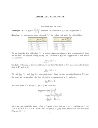
5. LIMITS AND CONTINUITY 5
(e) lim
x→3
f(x)
Solution.
The graph is shown below.
And,
(a) lim
x→0−
f(x) = lim
x→0−
x3
− 1 = −1
(b) lim
x→0+
f(x) = lim
x→0+
√
x + 1 − 2 = −1
(c) lim
x→0
f(x) = −1
(d) lim
x→−1
f(x) = lim
x→−1
x3
− 1 = −2
(e) lim
x→3
f(x) = lim
x→3
√
x + 1 − 2 = 0
2. Computation of Limits
It is easy to see that for any constant c and any real number a,
lim
x→a
c = c,
and
lim
x→a
x = a.
The following theorem lists some basic rules for dealing with common limit problems
Theorem 2.1 Suppose that lim
x→a
f(x) and lim
x→a
g(x) both exist and let c be any constant. Then,
(i) lim
x→a
[cf(x)] = c lim
x→a
f(x),
(ii) lim
x→a
[f(x) ± g(x)] = lim
x→a
f(x) ± lim
x→a
g(x),
(iii) lim
x→a
[f(x)g(x)] = lim
x→a
f(x) lim
x→a
g(x) , and
(iv) lim
x→a
f(x)
g(x)
=
lim
x→a
f(x)
lim
x→a
g(x)
provided lim
x→a
g(x) = 0.
By using (iii) of Theorem 2.1, whenever lim
x→a
f(x) exits,
lim
x→a
[f(x)]2
= lim
x→a
[f(x)f(x)]
= lim
x→a
f(x) lim
x→a
f(x) = lim
x→a
f(x)
2
.
Repeating this argument, we get that
lim
x→a
[f(x)]2
= lim
x→a
f(x)
n
,
for any positive integer n. In particular, for any positive integer n and any real number a,
lim
x→a
xn
= an
.
Example 2.1. Evaluate
(1) lim
x→2
(3x2
− 5x + 4).

6. 6 LIMITS AND CONTINUITY
(2) lim
x→3
x3
− 5x + 4
x2 − 2
.
(3) lim
x→1
x2
− 1
1 − x
.
Theorem 2.2 For any polynomial p(x) and any real number a,
lim
x→a
p(x) = p(a).
Theorem 2.3 Suppose that lim
x→a
f(x) = L and n is any positive integer. Then,
lim
x→a
n
f(x) = n lim
x→a
f(x) =
n
√
L,
where for n even, we assume that L > 0.
Example 2.2. Evaluate
(1) lim
x→2
5
√
3x2 − 2x.
(2) lim
x→0
√
x + 2 −
√
2
x
.
Theorem 2.4 For any real number a, we have
(i) lim
x→a
sin x = sin a,
(ii) lim
x→a
cos x = cos a,
(iii) lim
x→a
ex
= ea
,
(iv) lim
x→a
ln x = ln a, for a > 0,
(v) lim
x→a
sin−1
x = sin−1
a, for −1 < a < 1,
(vi) lim
x→a
cos−1
x = cos−1
a, for −1 < a < 1,
(vii) lim
x→a
tan−1
x = tan−1
a, for −∞ < a < ∞,
(viii) if p is a polynomial and lim
x→p(a)
f(x) = L, then lim
x→a
f(p(x)) = L.
Example 2.3. Evaluate lim
x→0
sin−1 x + 1
2
.
Example 2.4. Evaluate lim
x→0
(x cot x).
Theorem 2.5 (Sandwich Theorem) Suppose that
f(x) ≤ g(x) ≤ h(x)
for all x in some interval (c, d), except possibly at the point a ∈ (c, d) and that
lim
x→a
f(x) = lim
x→a
h(x) = L,
for some number L. Then, it follows that
lim
x→a
g(x) = L, too.

7. LIMITS AND CONTINUITY 7
Example 2.5. Evaluate lim
x→0
x2
cos
1
x
.
Example 2.6. Evaluate lim
x→0
f(x), where f is defined by
f(x) =
x2
+ 2 cos x + 1 if x < 0
ex
− 4 if x ≥ 0
.
Example 2.7. Evaluate.
(1) lim
x→0
1 − e2x
1 − ex
.
(2) lim
x→1
x3
− 1
x2 + 2x − 3
.
(3) lim
x→0
sin x
tan x
.
(4) lim
x→0
tan 2x
5x
.
(5) lim
x→0
xe−2x+1
x2 + x
.
(6) lim
x→0+
x2
csc2
x.
(7) lim
x→1
1
x − 1
−
2
x2 − 1
.
(8) lim
x→0
(1 + x)3
− 1
x
.
(9) lim
x→0
sin |x|
x
.
(10) lim
x→1
x .
(11) lim
x→1.5
x .
(12) lim
x→1
(x − x ).
3. Continuity and Its Consequences
A function f is continuous at x = a when
(i) f(a) is defined,
(ii) lim
x→a
f(x) exists, and
(iii) lim
x→a
f(x) = f(a).
Otherwise f is said to be discontinuous at x = a.
Example 3.1. Let us see some examples of functions that are discontinuous at x = a.
(1) The function is not defined at x = a. The graph has a hole at x = a.

8. 8 LIMITS AND CONTINUITY
(2) The function is defined at x = a, but lim
x→a
f(x) does not exist. The graph has a jump at
x = a.
(3) lim
x→a
f(x) exists and f(a) is defined but lim
x→a
f(x) = f(a). The graph has a hole at x = a.
(4) lim
x→a
f(x) = ∞ and so lim
x→a
f(x) = f(a) never holds. The function blows up at x = a.
Example 3.2. Determine where f(x) =
x2
+ 2x − 3
x − 1
is continuous.
The point x = a is called a removable discontinuity of a function f if one can remove the
discontinuity by redefining the function at that point. Otherwise, it is called a nonremovable
or an essential discontinuity of f. Clearly, a function has a removable discontinuity at x = a if
and only if lim
x→a
f(x) exists and is finite.

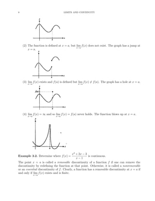
9. LIMITS AND CONTINUITY 9
Example 3.3. Classify all the discontinuities of
(1) f(x) =
x2
+ 2x − 3
x − 1
.
(2) f(x) =
1
x2
.
(3) f(x) = cos
1
x
.
Theorem 3.1 All polynomials are continuous everywhere. Additionally, sin x, cos x, tan−1
x
and ex
are continuous everywhere, n
√
x is continuous for all x, when n is odd and for x > 0, when
n is even. We also have ln x is continuous for x > 0 and sin−1
x and cos−1
x are continuous
for −1 < x < 1.
Theorem 3.2 Suppose that f and g are continuous at x = a. Then all of the following are
true:
(1) (f ± g) is continuous at x = a,
(2) (f · g) is continuous at x = a, and
(3) (f/g) is continuous at x = a if g(a) = 0.
Example 3.4. Find and classify all the discontinuities of
x4
− 3x2
+ 2
x2 − 3x − 4
.
Theorem 3.3 Suppose that lim
x→a
g(x) = L and f is continuous at L. Then,
lim
x→a
f(g(x)) = f lim
x→a
g(x) = f(L).
Corollary 3.4 Suppose that g is continuous at a and f is continuous at g(a). Then the
composition f ◦ g is continuous at a.
Example 3.5. Determine where h(x) = cos(x2
− 5x + 2) is continuous.
If f is continuous at every point on an open interval (a, b), we say that f is continuous on (a, b).
We say that f is continuous on the closed interval [a, b], if f is continuous on the open interval
(a, b) and
lim
x→a+
f(x) = f(a) and lim
x→b−
f(x) = f(b).
Finally, if f is continuous on all of (−∞, ∞), we simply say that f is continuous.
Example 3.6. Determine the interval(s) where f is continuous, for
(1) f(x) =
√
4 − x2,
(2) f(x) = ln(x − 3).
Example 3.7. For what value of a is
f(x) =
x2
− 1, x < 3
2ax, x ≥ 3
continuous at every x?

10. 10 LIMITS AND CONTINUITY
Example 3.8. Let
f(x) =



2 sgn(x − 1), x > 1,
a, x = 1,
x + b, x < 1.
If f is continuous at x = 1, find a and b.
Theorem 3.5 (Intermediate Value Theorem) Suppose that f is continuous on the closed in-
terval [a, b] and W is any number between f(a) and f(b). Then, there is a number c ∈ [a, b] for
which f(c) = W.
Example 3.9. Two illustrations of the intermediate value theorem:
Corollary 3.6 Suppose that f is continuous on [a, b] and f(a) and f(b) have opposite signs.
Then, there is at least one number c ∈ (a, b) for which f(c) = 0.
4. Limits involving infinity; asymptotes
If the values of f grow without bound, as x approaches a , we say that limx→a f(x) = ∞.
Similarly, if the values of f become arbitrarily large and negative as x approaches a, we say
that lim
x→a
f(x) = −∞.
A line x = a is a vertical asymptote of the graph of a function y = f(x) if either
lim
x→a+
f(x) = ±∞ or lim
x→a−
f(x) = ±∞.
Example 4.1. Evaluate
(1) lim
x→0
1
x
.
(2) lim
x→−3
1
(x + 3)2
.
(3) lim
x→2
(x − 2)2
x2 − 4
.
(4) lim
x→2
x − 2
x2 − 4
.
(5) lim
x→2+
x − 3
x2 − 4
.

11. LIMITS AND CONTINUITY 11
(6) lim
x→2−
x − 3
x2 − 4
.
(7) lim
x→2
x − 3
x2 − 4
.
(8) lim
x→2
2 − x
(x − 2)3
.
(9) lim
x→5
1
(x − 5)3
.
(10) lim
x→−2
x + 1
(x − 3)(x + 2)
.
(11) lim
x→ π
2
tan x.
Intuitively, limx→∞ f(x) = L (or, limx→−∞ f(x) = L if x moves increasingly far from the origin
in the positive direction (or, in the negative direction), f(x) gets arbitrarily close to L.
Example 4.2. Clearly, lim
x→∞
1
x
= 0 and lim
x→−∞
1
x
= 0.
A line y = b is a horizontal asymptote of the graph of a function y = f(x) if either
lim
x→∞
f(x) = b or lim
x→−∞
f(x) = b.
Example 4.3. Evaluate lim
x→∞
5 +
1
x
.
Theorem 4.1 For any rational number t > 0,
lim
x→±∞
1
xt
= 0,
where for the case where x → −∞, we assume that t = p/q where q is odd.
Theorem 4.2 For any polynomial of degree n > 0, pn(x) = anxn
+ an−1xn−1
+ · · · + a0, we
have
lim
x→∞
pn(x) =
∞ if an > 0
−∞ if an < 0
Example 4.4. Evaluate
(1) lim
x→∞
2x3
+ 7
x3 − x2 + x + 7
.
(2) lim
x→∞
3x + 7
x2 − 2
.
(3) lim
x→∞
sin
1
x
.
(4) lim
x→∞
√
x2 + 2x + 3 − x.
(5) lim
x→∞
sin x
x
.
(6) lim
x→∞
sin x.
Example 4.5. Find the horizontal asymptote(s) of f(x) =
2 − x + sin x
x + cos x

12. 12 LIMITS AND CONTINUITY
Let f(x) =
P(x)
Q(x)
. If (the degree of P) = (the degree of Q)+1, then the graph of f has a
oblique (slant) asymptote. We find an equation for the asymptote by dividing numerator by
denominator to express f as a linear function plus a remainder that goes to 0 as x → ±∞.
Example 4.6. Find the asymptotes of the graph of f, if
(1) f(x) =
x2
− 3
2x − 4
.
(2) f(x) =
2x
x + 1
.
Example 4.7. Evaluate
(1) lim
x→0−
e
1
x .
(2) lim
x→0+
e
1
x .
(3) lim
x→∞
tan−1
x.
(4) lim
x→−∞
tan−1
x.
(5) lim
x→0+
ln x.
(6) lim
x→∞
ln x.
(7) lim
x→0
sin e
− 1
x2
.
(8) lim
x→∞
x
√
x2 + 1
.
(9) lim
x→−∞
x
√
x2 + 1
.