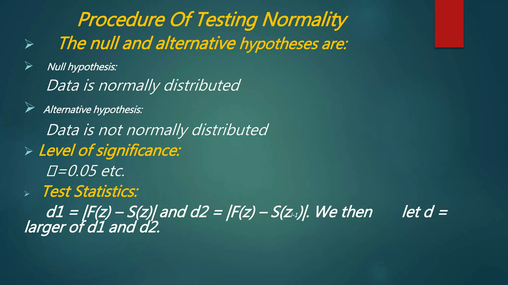
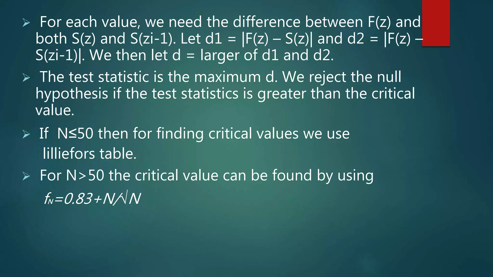
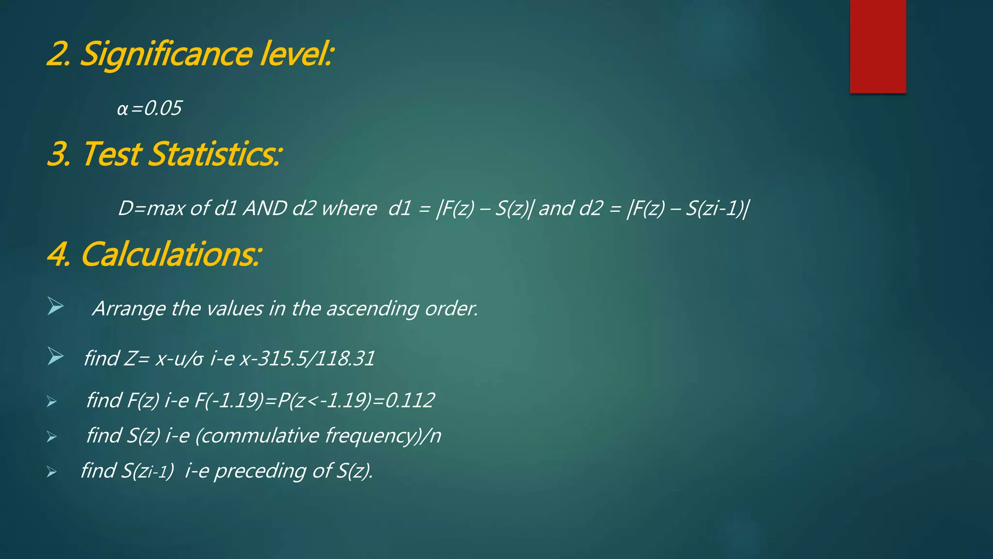
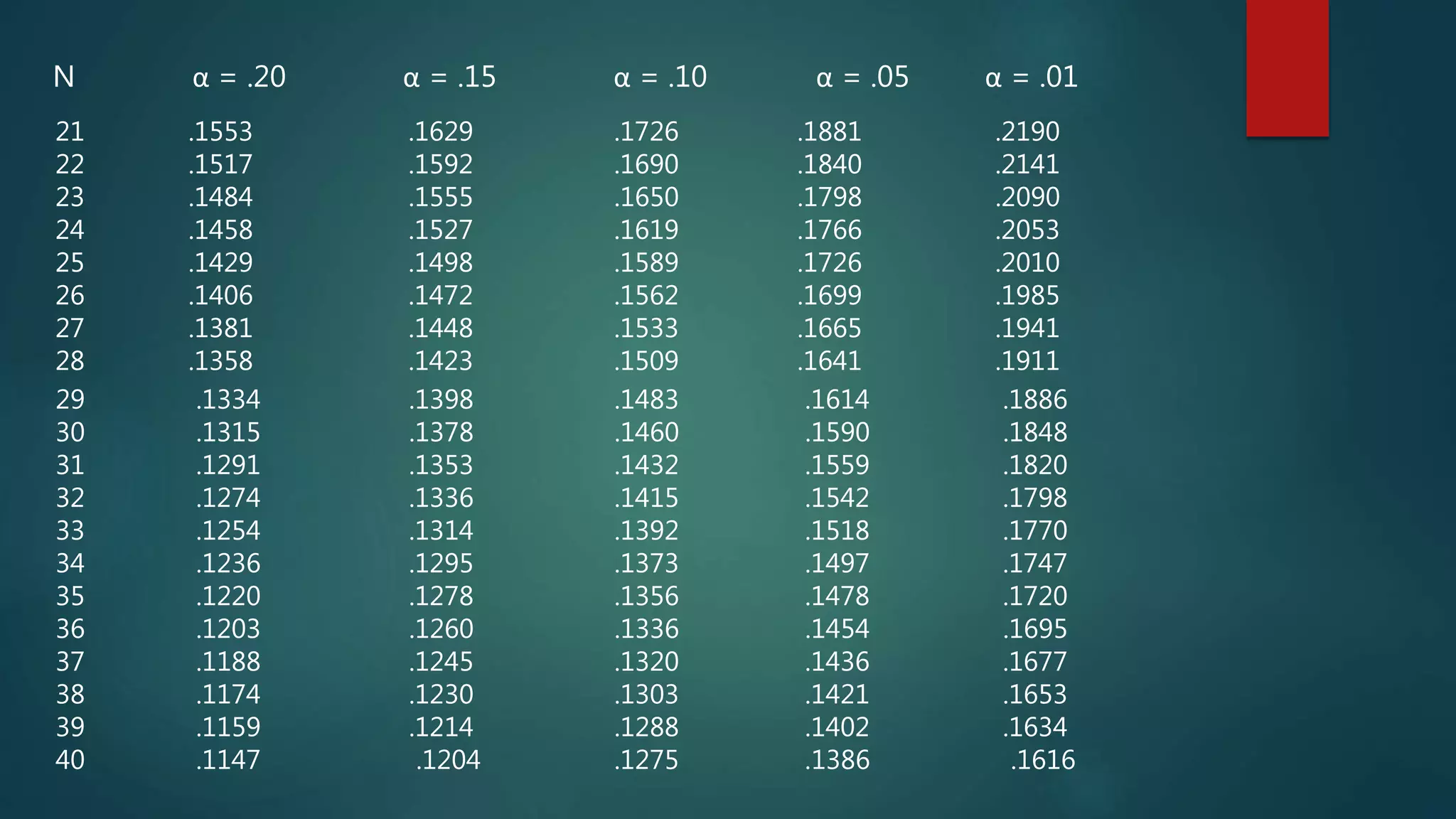
The document provides information about the Lilliefors test for normality. It discusses that the Lilliefors test was derived in 1967 by Hubert Lilliefors and is used to test the null hypothesis that data comes from a normal distribution based on the Kolmogorov-Smirnov test. It then outlines the procedure for conducting the Lilliefors test, which includes determining the test statistic by calculating the maximum difference between the empirical distribution function and the theoretical normal distribution function, and comparing this value to critical values from a table to determine whether to reject or fail to reject the null hypothesis. An example applying the Lilliefors test to sample data is also provided and worked through step

1. In the name of Allah, the
most Merciful and the
most Almighty.

2. TOPIC:-
Lilliefors test for normality

3. About Hubert Whitman Lilliefors:
 Hubert Whitman Lilliefors (born on February 23-1928, and died in 2008, at
Bethesda, Maryland). He was an American statistician, noted for his
introduction of the Lilliefors test. He was a professor of statistics at George
Washington University for 39 years, and also obtained his PhD there in
1964 under the supervision of Solomon Kullback.

4. Introduction:
 Lilliefors test is derived in 1967 by Hubert Lilliefors.
 It is used to test the null hypothesis that data comes
from normal distribution.
 It is based on the Kolmogorov-Smirnov test of
normality.
Assumption:
 The sample is a random sample.

5. Procedure Of Testing Normality
 The null and alternative hypotheses are:
 Null hypothesis:
Data is normally distributed
 Alternative hypothesis:
Data is not normally distributed
 Level of significance:
=0.05 etc.
 Test Statistics:
d1 = |F(z) – S(z)| and d2 = |F(z) – S(zi-1)|. We then let d =
larger of d1 and d2.

6. Procedure for the test statistic
 Sort the data from lowest to highest.
 Compute the sample mean and the sample standard
deviation and for each value of X, compute Z .
 For each value, compute F(z) which is the left-tail
probability of Z.
 For each value, compute S(z) and S(zi-1).

7.  For each value, we need the difference between F(z) and
both S(z) and S(zi-1). Let d1 = |F(z) – S(z)| and d2 = |F(z) –
S(zi-1)|. We then let d = larger of d1 and d2.
 The test statistic is the maximum d. We reject the null
hypothesis if the test statistics is greater than the critical
value.
 If N≤50 then for finding critical values we use
lilliefors table.
 For N>50 the critical value can be found by using
fN=0.83+N/√N

8. Critical region:
Dcal≥ Dtab, then reject H0.
Conclusion:

9.  Example:
 A store wanted to determine if the average sale is significantly more than $250. A random
sample had the following results:
 Test at a 5% level of significance.

 Solution:
 NULL AD ALTERNATIVE hypothesis:
H0: Data is normally distributed.
H1: Data is not normally distributed.

10. 2. Significance level:
α=0.05
3. Test Statistics:
D=max of d1 AND d2 where d1 = |F(z) – S(z)| and d2 = |F(z) – S(zi-1)|
4. Calculations:
 Arrange the values in the ascending order.
 find Z= x-u/σ i-e x-315.5/118.31
 find F(z) i-e F(-1.19)=P(z<-1.19)=0.112
 find S(z) i-e (commulative frequency)/n
 find S(zi-1) i-e preceding of S(z).

11. X F C.F z P(z) F(z) S(zi) S(zi-1) D1=│F(z)-
S(z)│
D2=│F(z)-S(zi-
1)│
175 1 1 -1.19 0.3880 0.112 1/12=0.083 0 0.112-0.083=0.029 0.122-0=0.122
189 1 2 -1.07 0.3577 0.1423 2/12=0.166 1/12=0.083 0.1423-0.016=0.1257 0.1423-0.083=0.0653
200 1 3 -0.98 0.3365 0.1635 3/12=0.25 2/12=0.166 0.1635-0.25=0.086 0.0025
212 1 4 -0.87 0.3078 0.1922 4/12=0.333 3/12=0.25 0.1922-0.333=0.140 0.578
262 1 5 -0.45 0.1736 0.3264 5/12=0.416 4/12=0.333 0.3264-0.416=0.089 0.0066
298 1 6 -0.15 0.0596 0.4404 6/12=0.5 5/12=0.416 0.4404-0.5=0.0596 0.0244
325 1 7 0.08 0.0319 0.5319 7/12=0.583 6/12=0.5 0.0511 0.0319
355 1 8 0.33 0.1293 0.3707 8/12=0.667 7/12=0.583 0.2963 0.2123
360 1 9 0.38 0.1480 0.352 9/12=0.751 8/12=0.667 0.399 0.315
410 1 10 0.79 0.2852 0.2148 10/12=0.83 9/12=0.751 0.6125 0.5362
428 1 11 0.95 0.3289 0.1711 11/12=0.91 10/12=0.83 0.7389 0.6589
572 1 12 2.17 0.4850 0.015 12/12= 1 11/12=0.91 0.985 0.895

12. 5. Critical value:
If Dcal ≥ Table values ;
then we reject our null hypothesis.
DCAL =0.985 , Table value = 0.2426
6. Conclusion:
Since the calculated value of D is greater than the table value therefore
we reject our null hypothesis and conclude that data is not
normally distributed.

13. Example# 2
 An Independent random samples from 6 assistant professors. They asked about their time
used outside the class in the last week. Data is shown below (in hours)
7, 12, 11, 15, 9, 14.
Solution:
1. Hypothesis would be:
H0: the data are normally distributed
H1: the data are not normally distributed

14. 2. Significance level:
α=0.05
3. Test Statistics:
D=max of d1 AND d2 where d1 = |F(z) – S(z)| and d2 = |F(z) – S(zi-1)|
4. Calculations:
 Arrange the values in the ascending order.
 find Z= x-u/σ i-e x-11.3333/3.0111
 find F(z) i-e F(-1.44)=P(z<-1.44)=0.0764
 find S(z) i-e (commulative frequency)/n
 find S(zi-1) i-e preceding of S(z).

15. X Z P(z) F(z) S(zi) S(zi-1) D1=│F(z)-
S(z)│
D2=│F(z)-
S(zi-1)│
7 -1.44 0.4251 0.0764 0.1666 0 0.0764-0.1666=
0.0902
0.0764-0=
0.0764
9 -0.77 0.2794 0.2206 0.3333 0.1666 0.1127 0.2206-
0.1666=
0.054
11 -0.11 0.0438 0.4562 0.5000 0.3333 0.0438 0.1229
12 0.22 0.0871 0.5871 0.6667 0.5000 0.0796 0.0871
14 0.89 0.3133 0.8133 0.8333 0.6667 0.0200 0.1466
15 1.22 0.3888 0.8888 1 0.8333 0.1112 0.0555

16. 5. Critical value:
If Dcal ≥Table values ;
then we reject our null hypothesis.
DCAL =0.1127 , Table value = 0.2426
6. Conclusion:
Since the calculated value of D is less than the table value therefore
we do not reject our null hypothesis and conclude that data is
normally distributed.

17. Critical values :
N α = .20 α = .15 α = .10 α = .05 α = .01
4 .3027 .3216 .3456 .3754 .4129
5 .2893 .3027 .3188 .3427 .3959
6 .2694 .2816 .2982 .3245 .3728
7 .2521 .2641 .2802 .3041 .3504
8 .2387 .2502 .2649 .2875 .3331
9 .2273 .2382 .2522 .2744 .3162
10 .2171 .2273 .2410 .2616 .3037
11 .2080 .2179 .2306 .2506 .2905
12 .2004 .2101 .2228 .2426 .2812
13 .1932 .2025 .2147 .2337 .2714
14 .1869 .1959 .2077 .2257 .2627
15 .1811 .1899 .2016 .2196 .2545
16 .1758 .1843 .1956 .2128 .2477
17 .1711 .1794 .1902 .2071 .2408
18 .1666 .1747 .1852 .2018 .2345
19 .1624 .1700 .1803 .1965 .2285
20 .1589 .1666 .1764 .1920 .2226

18. N α = .20 α = .15 α = .10 α = .05 α = .01
21 .1553 .1629 .1726 .1881 .2190
22 .1517 .1592 .1690 .1840 .2141
23 .1484 .1555 .1650 .1798 .2090
24 .1458 .1527 .1619 .1766 .2053
25 .1429 .1498 .1589 .1726 .2010
26 .1406 .1472 .1562 .1699 .1985
27 .1381 .1448 .1533 .1665 .1941
28 .1358 .1423 .1509 .1641 .1911
29 .1334 .1398 .1483 .1614 .1886
30 .1315 .1378 .1460 .1590 .1848
31 .1291 .1353 .1432 .1559 .1820
32 .1274 .1336 .1415 .1542 .1798
33 .1254 .1314 .1392 .1518 .1770
34 .1236 .1295 .1373 .1497 .1747
35 .1220 .1278 .1356 .1478 .1720
36 .1203 .1260 .1336 .1454 .1695
37 .1188 .1245 .1320 .1436 .1677
38 .1174 .1230 .1303 .1421 .1653
39 .1159 .1214 .1288 .1402 .1634
40 .1147 .1204 .1275 .1386 .1616

19. N α = .20 α = .15 α = .10 α = .05 α = .01
41 .1131 .1186 .1258 .1373 .1599
42 .1119 .1172 .1244 .1353 .1573
43 .1106 .1159 .1228 .1339 .1556
44 .1095 .1148 .1216 .1322 .1542
45 .1083 .1134 .1204 .1309 .1525
46 .1071 .1123 .1189 .1293 .1512
47 .1062 .1113 .1180 .1282 .1499
48 .1047 .1098 .1165 .1269 .1476
49 .1040 .1089 .1153 .1256 .1463
50 .1030 .1079 .1142 .1246 .1457
 50 0.741/fN 0.775/fN 0.819/fN 0.895/fN 1.035/fN
 Where f(n)=
𝟎.𝟖𝟑+𝒏
√𝒏
− 𝟏

20. THANK YOU 