2/12/2013
1
Testing for Normality
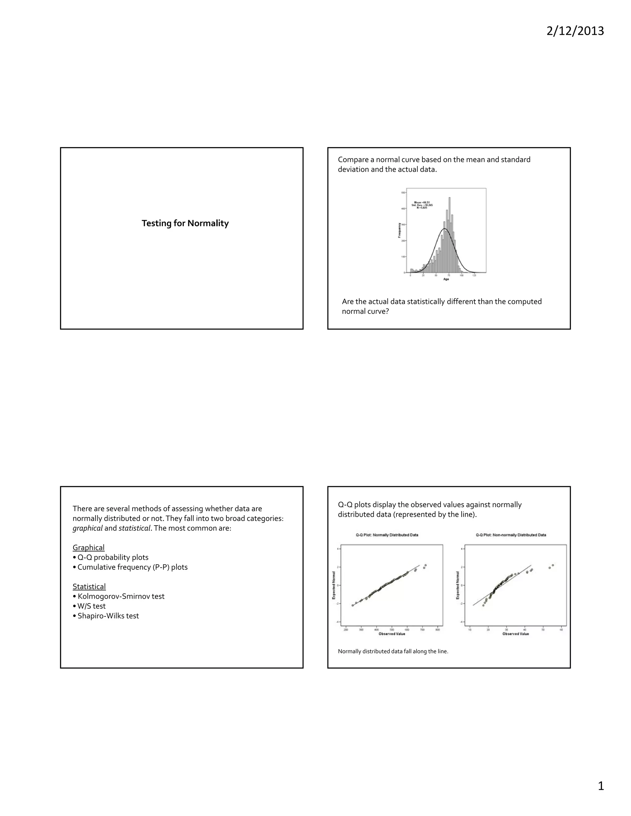
Compare a normal curve based on the mean and standard 
deviation and the actual data.
Are the actual data statistically different than the computed 
normal curve?
There are several methods of assessing whether data are 
normally distributed or not. They fall into two broad categories: 
graphical and statistical. The most common are:
Graphical
• Q‐Q probability plots
• Cumulative frequency (P‐P) plots
Statistical
• Kolmogorov‐Smirnov test
•W/S test
• Shapiro‐Wilks test
Q‐Q plots display the observed values against normally 
distributed data (represented by the line).
Normally distributed data fall along the line.
2/12/2013
2
Tests of Normality
.110 1048 .000 .931 1048 .000Age
Statistic df Sig. Statistic df Sig.
Kolmogorov-Smirnov
a
Shapiro-Wilk
Lilliefors Significance Correctiona.
Tests of Normality
.283 149 .000 .463 149 .000TOTAL_VALU
Statistic df Sig. Statistic df Sig.
Kolmogorov-Smirnov
a
Shapiro-Wilk
Lilliefors Significance Correctiona.
Tests of Normality
.071 100 .200* .985 100 .333Z100
Statistic df Sig. Statistic df Sig.
Kolmogorov-Smirnov
a
Shapiro-Wilk
This is a lower bound of the true significance.*.
Lilliefors Significance Correctiona.
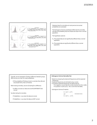
Statistical tests for normality are more precise since actual 
probabilities are calculated.
The Kolmogorov‐Smirnov and Shapiro‐Wilks tests for normality
calculate the probability that the sample was drawn from a normal
population.
The hypotheses used are:
H0: The sample data are not significantly different than a normal 
population.
Ha: The sample data are significantly different than a normal 
population.
Typically, we are interested in finding a difference between groups.
When we are, we ‘look’ for small probabilities.
• If the probability of finding an event is rare (less than 5%) and
we actually find it, that is of interest.
When testing normality, we are not looking for a difference.
• In effect, we want our data set to be NO DIFFERENT than
normal.
So when testing for normality:
• Probabilities > 0.05 mean the data are normal.
• Probabilities < 0.05 mean the data are NOT normal.
Kolmogorov‐Smirnov Normality Test
• Based on comparing the observed frequencies and the expected
frequencies.
• Expected frequencies are estimated using z‐scores.
• Cumulative expected frequencies are determined as:
• For negative z‐scores take the number directly from the z‐table.
• For positive z‐scores use (1 ‐ the z‐score from the table).
Kolmogorov‐Smirnov D statistic:
iii
iii
FrelFrelD
and
FrelFrelD
ˆ
ˆ
1
'



Use absolute values.
2/12/2013
3
Height
(in)
Observed
Frequency
Cumulative
Observed
Frequency
Cumulative
Relative Observed
Frequency (Fi)
62 0 0 (0 / 70) 0.0000
63 2 2 (2 / 70) 0.0286
64 2 4 (4 / 70) 0.0571
65 3 7 . 0.1000
66 5 12 . 0.1714
67 4 16 . 0.2286
68 6 22 . 0.3143
69 5 27 . 0.3857
70 8 35 . 0.5000
71 7 42 . 0.6000
72 7 49 . 0.7000
73 10 59 . 0.8429
74 6 65 . 0.9286
75 3 68 . 0.9714
76 2 70 . 1.0000
77 0 70 . 1.0000
78 0 70 . 1.0000
Mean = 70.17
Standard deviation = 3.31
n = 70
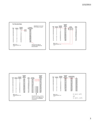
Important: Sort the data
from smallest to largest.
For Discrete Data:
These are also called the
cumulative percentages and
will be used later.
Height
(in)
Observed
Frequency
Cumulative
Observed
Frequency
Cumulative
Relative
Observed
Frequency
(Fi)
Z-score
Calculation
Height
Z-score
62 0 0 0.0000 (62 – 70.17) / 3.31 -2.47
63 2 2 0.0286 (63 – 70.17) / 3.31 -2.17
64 2 4 0.0571 (64 – 70.17) / 3.31 -1.86
65 3 7 0.1000 . -1.56
66 5 12 0.1714 . -1.26
67 4 16 0.2286 . -0.96
68 6 22 0.3143 . -0.66
69 5 27 0.3857 . -0.35
70 8 35 0.5000 . -0.05
71 7 42 0.6000 . 0.25
72 7 49 0.7000 . 0.55
73 10 59 0.8429 . 0.85
74 6 65 0.9286 . 1.16
75 3 68 0.9714 . 1.46
76 2 70 1.0000 . 1.76
77 0 70 1.0000 . 2.06
78 0 70 1.0000 . 2.37
Mean = 70.17
Standard deviation = 3.31
n = 70
Height
(in)
Observed
Frequency
Cumulative
Observed
Frequency
Cumulative
Relative
Observed
Frequency
(Fi)
Height
Z-score
Probability
from Z-Table
Cumulative
Relative
Expected
Frequency
(F-hati)
62 0 0 0.0000 -2.47 0.0068 . 0.0068
63 2 2 0.0286 -2.17 0.0150 . 0.0150
64 2 4 0.0571 -1.86 0.0314 . 0.0314
65 3 7 0.1000 -1.56 0.0594 . 0.0594
66 5 12 0.1714 -1.26 0.1038 . 0.1038
67 4 16 0.2286 -0.96 0.1736 . 0.1736
68 6 22 0.3143 -0.66 0.2546 . 0.2546
69 5 27 0.3857 -0.35 0.3632 . 0.3632
70 8 35 0.5000 -0.05 0.4801 . 0.4801
71 7 42 0.6000 0.25 0.4013 (1 – 0.4013) 0.5987
72 7 49 0.7000 0.55 0.2912 (1 – 0.2912) 0.7088
73 10 59 0.8429 0.85 0.1977 (1 – 0.1977) 0.8023
74 6 65 0.9286 1.16 0.1230 (1 – 0.1230) 0.8770
75 3 68 0.9714 1.46 0.0721 (1 – 0.0721) 0.9279
76 2 70 1.0000 1.76 0.0392 (1 – 0.0392) 0.9608
77 0 70 1.0000 2.06 0.0197 (1 – 0.0197) 0.9803
78 0 70 1.0000 2.37 0.0089 (1 – 0.0089) 0.9911
Mean = 70.17
Standard deviation = 3.31
n = 70 Remember to use (1 – p) for all
positive z‐scores. Only use (1‐p) 
when calculating cumulative
probabilities!
Height
(in)
Observed
Frequency
Cumulative
Observed
Frequency
Cumulative
Relative
Observed
Frequency (Fi)
Cumulative Relative
Expected Frequency
(F-hati) Di
62 0 0 0.0000 0.0068 0.0068
63 2 2 0.0286 0.0150 0.0136
64 2 4 0.0571 0.0314 0.0257
65 3 7 0.1000 0.0594 0.0406
66 5 12 0.1714 0.1038 0.0676
67 4 16 0.2286 0.1736 0.0550
68 6 22 0.3143 0.2546 0.0597
69 5 27 0.3857 0.3632 0.0225
70 8 35 0.5000 0.4801 0.0199
71 7 42 0.6000 0.5987 0.0013
72 7 49 0.7000 0.7088 0.0088
73 10 59 0.8429 0.8023 0.0406
74 6 65 0.9286 0.8770 0.0516
75 3 68 0.9714 0.9279 0.0435
76 2 70 1.0000 0.9608 0.0392
77 0 70 1.0000 0.9803 0.0197
78 0 70 1.0000 0.9911 0.0089
Mean = 70.17
Standard deviation = 3.31
n = 70
iii
iii
FrelFrelD
and
FrelFrelD
ˆ
ˆ
1
'



2/12/2013
4
Height
(in)
Observed
Frequency
Cumulative
Observed
Frequency
Cumulative
Relative
Observed
Frequency (Fi)
Cumulative Relative
Expected Frequency
(F-hati) Di D’i
62 0 0 0.0000 0.0068 0.0068 0.0068
63 2 2 0.0286 0.0150 0.0136 0.0150
64 2 4 0.0571 0.0314 0.0257 0.0028
65 3 7 0.1000 0.0594 0.0406 0.0023
66 5 12 0.1714 0.1038 0.0676 0.0038
67 4 16 0.2286 0.1736 0.0550 0.0022
68 6 22 0.3143 0.2546 0.0597 0.0260
69 5 27 0.3857 0.3632 0.0225 0.0489
70 8 35 0.5000 0.4801 0.0199 0.0944
71 7 42 0.6000 0.5987 0.0013 0.0987
72 7 49 0.7000 0.7088 0.0088 0.1088
73 10 59 0.8429 0.8023 0.0406 0.1023
74 6 65 0.9286 0.8770 0.0516 0.0341
75 3 68 0.9714 0.9279 0.0435 0.0007
76 2 70 1.0000 0.9608 0.0392 0.0106
77 0 70 1.0000 0.9803 0.0197 0.0197
78 0 70 1.0000 0.9911 0.0089 0.0089
Mean = 70.17
Standard deviation = 3.31
n = 70
iii
iii
FrelFrelD
and
FrelFrelD
ˆ
ˆ
1
'



Height
(in)
Observed
Frequency
Cumulative
Observed
Frequency
Cumulative
Relative
Observed
Frequency (Fi)
Cumulative Relative
Expected Frequency
(F-hati) Di D’i
62 0 0 0.0000 0.0068 0.0068 0.0068
63 2 2 0.0286 0.0150 0.0136 0.0150
64 2 4 0.0571 0.0314 0.0257 0.0028
65 3 7 0.1000 0.0594 0.0406 0.0023
66 5 12 0.1714 0.1038 0.0676 0.0038
67 4 16 0.2286 0.1736 0.0550 0.0022
68 6 22 0.3143 0.2546 0.0597 0.0260
69 5 27 0.3857 0.3632 0.0225 0.0489
70 8 35 0.5000 0.4801 0.0199 0.0944
71 7 42 0.6000 0.5987 0.0013 0.0987
72 7 49 0.7000 0.7088 0.0088 0.1088
73 10 59 0.8429 0.8023 0.0406 0.1023
74 6 65 0.9286 0.8770 0.0516 0.0341
75 3 68 0.9714 0.9279 0.0435 0.0007
76 2 70 1.0000 0.9608 0.0392 0.0106
77 0 70 1.0000 0.9803 0.0197 0.0197
78 0 70 1.0000 0.9911 0.0089 0.0089
Mean = 70.17
Standard deviation = 3.31
n = 70
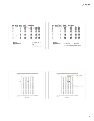
Di Max = 0.0676            D’i Max = 0.1088
D = 0.1088     (Use the larger of the 2 values)
Our calculated D value
falls about here.
Our probability falls
within this range.
2/12/2013
5
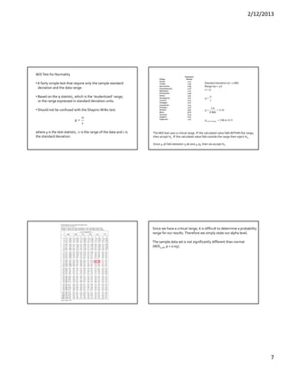
Dcritical = 0.106
D = 0.108
Since  0.108 > 0.106  reject Ho.
The sample data set is significantly different than normal (D0.05, 0.108, 0.05 > p > 0.025)
From SPSS:
Tests of Normality
.110 70 .036 .965 70 .045VAR00001
Statistic df Sig. Statistic df Sig.
Kolmogorov-Smirnov
a
Shapiro-Wilk
Lilliefors Significance Correctiona.
Non-Normally Distributed Data
.142 72 .001 .841 72 .000Average PM10
Statistic df Sig. Statistic df Sig.
Kolmogorov-Smirnov
a
Shapiro-Wilk
Lilliefors Significance Correctiona.
Remember that LARGE probabilities denote normally distributed data.
Normally Distributed Data
.069 72 .200* .988 72 .721Asthma Cases
Statistic df Sig. Statistic df Sig.
Kolmogorov-Smirnov
a
Shapiro-Wilk
This is a lower bound of the true significance.*.
Lilliefors Significance Correctiona.
In this case the probabilities are greater than 0.05 (the typical alpha 
level), so we accept H0… these data are not different from normal.
Normally Distributed Data
.069 72 .200* .988 72 .721Asthma Cases
Statistic df Sig. Statistic df Sig.
Kolmogorov-Smirnov
a
Shapiro-Wilk
This is a lower bound of the true significance.*.
Lilliefors Significance Correctiona.
Non-Normally Distributed Data
.142 72 .001 .841 72 .000Average PM10
Statistic df Sig. Statistic df Sig.
Kolmogorov-Smirnov
a
Shapiro-Wilk
Lilliefors Significance Correctiona.
In this case the probabilities are less than 0.05 (the typical alpha level), 
so we reject H0… these data are significantly different from normal.
Important: As the sample size increases, normality parameters becomes 
MORE restrictive and it becomes harder to declare that the data are
normally distributed.
2/12/2013
6
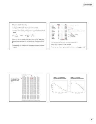
For Continuous Data:
Village
Population
Density
Observed
Cumulative
Frequency Z‐score
Z 
Probability
Expected
Cumulative
Frequency Di D'i
Aranza 4.13 0.0588 ‐1.40 0.0808 0.0808 0.0220 0.0808
Corupo 4.53 0.1176 ‐0.94 0.1736 0.1736 0.0560 0.1148
San Lorenzo                      4.69 0.1764 ‐0.75 0.2266 0.2266 0.0502 0.1090
Cheranatzicurin 4.76 0.2352 ‐0.67 0.2514 0.2514 0.0162 0.0750
Nahuatzen 4.77 0.2940 ‐0.66 0.2546 0.2546 0.0394 0.0194
Pomacuaran 4.96 0.3528 ‐0.44 0.3300 0.3300 0.0228 0.0360
Sevina 4.97 0.4116 ‐0.43 0.3336 0.3336 0.0780 0.0192
Arantepacua                      5.00 0.4704 ‐0.39 0.3483 0.3483 0.1221 0.0633
Cocucho 5.04 0.5292 ‐0.35 0.3632 0.3632 0.1660 0.1072
Charapan 5.10 0.5880 ‐0.28 0.3897 0.3897 0.1983 0.1395
Comachuen 5.25 0.6468 ‐0.10 0.4602 0.4602 0.1866 0.1278
Pichataro 5.36 0.7056 0.02 0.4920 0.5080 0.1976 0.1388
Quinceo 5.94 0.7644 0.69 0.2451 0.7549 0.0095 0.0493
Nurio 6.06 0.8232 0.83 0.2033 0.7967 0.0265 0.0323
Turicuaro 6.19 0.8820 0.98 0.1635 0.8365 0.0455 0.0133
Urapicho 6.30 0.9408 1.11 0.1335 0.8665 0.0743 0.0155
Capacuaro 7.73 0.9996 2.76 0.0029 0.9971 0.0025 0.0563
Mean = 5.34
SD = 0.866
N = 17
For the observed cumulative frequency simply
divide the observation by the sample size, so for
Aranza 1/17=0.0588, for Corupo 0.0588+0.0588=
0.1176, for San Lorenzo 0.0588+0.0588+0.0588=
0.1764, etc…
For Continuous Data:
Village
Population
Density
Observed
Cumulative
Frequency Z‐score
Z 
Probability
Expected
Cumulative
Frequency Di D'i
Aranza                           4.13 0.0588 ‐1.40 0.0808 0.0808 0.0220 0.0808
Corupo                           4.53 0.1176 ‐0.94 0.1736 0.1736 0.0560 0.1148
San Lorenzo                      4.69 0.1764 ‐0.75 0.2266 0.2266 0.0502 0.1090
Cheranatzicurin                  4.76 0.2352 ‐0.67 0.2514 0.2514 0.0162 0.0750
Nahuatzen                        4.77 0.2940 ‐0.66 0.2546 0.2546 0.0394 0.0194
Pomacuaran                       4.96 0.3528 ‐0.44 0.3300 0.3300 0.0228 0.0360
Sevina                           4.97 0.4116 ‐0.43 0.3336 0.3336 0.0780 0.0192
Arantepacua                      5.00 0.4704 ‐0.39 0.3483 0.3483 0.1221 0.0633
Cocucho                          5.04 0.5292 ‐0.35 0.3632 0.3632 0.1660 0.1072
Charapan                         5.10 0.5880 ‐0.28 0.3897 0.3897 0.1983 0.1395
Comachuen                        5.25 0.6468 ‐0.10 0.4602 0.4602 0.1866 0.1278
Pichataro                        5.36 0.7056 0.02 0.4920 0.5080 0.1976 0.1388
Quinceo                          5.94 0.7644 0.69 0.2451 0.7549 0.0095 0.0493
Nurio                            6.06 0.8232 0.83 0.2033 0.7967 0.0265 0.0323
Turicuaro                        6.19 0.8820 0.98 0.1635 0.8365 0.0455 0.0133
Urapicho                         6.30 0.9408 1.11 0.1335 0.8665 0.0743 0.0155
Capacuaro                        7.73 0.9996 2.76 0.0029 0.9971 0.0025 0.0563
Mean = 5.34
SD = 0.866
Di Max = 0.1983            D’i Max = 0.1395
D = 0.1983     (Use the larger of the 2 values)
Dcritical = 0.207 (from the table)
D = 0.1983 (computed)
Since  0.1983 < 0.207  accept Ho.
The sample data set is not significantly different than normal
(D0.05, 0.1983, 0.10 > p > 0.05)
From SPSS:
Tests of Normality
.197 17 .077 .883 17 .035VAR00001
Statistic df Sig. Statistic df Sig.
Kolmogorov-Smirnov
a
Shapiro-Wilk
Lilliefors Significance Correctiona.
Notice that there is disagreement between the Kolmogorov‐Smirnov and the Shapiro‐
Wilk tests.
2/12/2013
7
W/S Test for Normality
• A fairly simple test that require only the sample standard
deviation and the data range.
• Based on the q statistic, which is the ‘studentized’ range,
or the range expressed in standard deviation units.
• Should not be confused with the Shapiro‐Wilks test.
where q is the test statistic, w is the range of the data and s is 
the standard deviation.
s
w
q 
Village
Population
Density
Aranza 4.13
Corupo 4.53
San Lorenzo                      4.69
Cheranatzicurin 4.76
Nahuatzen 4.77
Pomacuaran 4.96
Sevina 4.97
Arantepacua                      5.00
Cocucho 5.04
Charapan 5.10
Comachuen 5.25
Pichataro 5.36
Quinceo 5.94
Nurio 6.06
Turicuaro 6.19
Urapicho 6.30
Capacuaro 7.73
Standard deviation (s) = 0.866
Range (w) = 3.6
n = 17
31.406.3
16.4
866.0
6.3
toq
q
s
w
q
RangeCritical 


The W/S test uses a critical range. IF the calculated value falls WITHIN the range,
then accept Ho. IF the calculated value falls outside the range then reject Ho.
Since 4.16 falls between 3.06 and 4.31, then we accept Ho.
Since we have a critical range, it is difficult to determine a probability 
range for our results. Therefore we simply state our alpha level.
The sample data set is not significantly different than normal 
(W/S4.16, p > 0.05).
2/12/2013
8
D’Agostino Test for Normality
• A very powerful test for departures from normality.
• Based on the D statistic, which gives an upper and lower critical
value.
where D is the test statistic, SS is the sum of squares of the data 
and n is the sample size, and i is the order or rank of observation
X.
• First the data are ordered from smallest to largest or largest to
smallest.
 




 
 iX
n
iTwhere
SSn
T
D
2
1
3
Village
Population
Density i
Mean
Deviates2
Aranza 4.13 1 1.46410
Corupo 4.53 2 0.65610
San Lorenzo                4.69 3 0.42250
Cheranatzicurin 4.76 4 0.33640
Nahuatzen 4.77 5 0.32490
Pomacuaran 4.96 6 0.14440
Sevina 4.97 7 0.13690
Arantepacua                5.00 8 0.11560
Cocucho 5.04 9 0.09000
Charapan 5.10 10 0.05760
Comachuen 5.25 11 0.00810
Pichataro 5.36 12 0.00040
Quinceo 5.94 13 0.36000
Nurio 6.06 14 0.51840
Turicuaro 6.19 15 0.72250
Urapicho 6.30 16 0.92160
Capacuaro 7.73 17 5.71210
Mean = 5.34 SS = 11.9916
2860.0,2587.0
26050.0
)9916.11)(17(
23.63
23.63
73.7)917(69.4)93(53.4)92(13.4)91(
)9(
9
2
117
2
1
3
1










CriticalD
D
T
T
XiT
n

If the calculated value falls within the critical range, accept Ho.
Since 0.2587 < D = 0.26050 < 0.2860   accept Ho.
The sample data set is not significantly different than normal (D0.26050, p > 0.05).
46410.121.1)34.513.4( 22

Use the next lower
n on the table if your
sample size is NOT
listed.
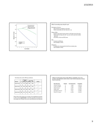
Values of D as Capacuaro’s
population density is increased.
Values of D as Aranza’s
population density is decreased.
2/12/2013
9
Decreasing Aranza’s
population density 
slightly made the data 
set more symmetrical.
Which normality test should I use?
Kolmogorov‐Smirnov: 
• Not sensitive to problems in the tails.
•Works reasonably well with data sets < 50.
Shapiro‐Wilks:
• Doesn't work well if several values in the data set are the same.
•Works best for data sets with > 50, but can be used with smaller 
data sets.
•The better of the two SPSS tests.
W/S:
• Simple, but effective.
• Not available in SPSS.
D’Agostino:
• Probably the most powerful of all the normality tests.
• Not available in SPSS.
Kolmogorov-
Smirnov Shapiro-Wilkes
Data Type N Statistic Prob Statistic Prob Q-QPlots
Random Normal 30 0.116 0.200 0.987 0.962
Random Normal 100 0.059 0.200 0.986 0.382
Random Normal 1000 0.019 0.200 0.998 0.386
Random Normal 2000 0.018 0.120 0.999 0.154
Normality tests under differing conditions
Notice that as the sample size increases, the probabilities decrease.
In other words, it gets harder to meet the normality assumption as 
the sample size increases since even small differences are detected.
Normality Test Statistic Calculated Value Probability
Anderson‐Darling A 1.0958 0.006219
Cramer‐von Mises W 0.1776 0.009396
Shapiro‐Francia W 0.9186 0.013690
Shapiro‐Wilk  W 0.9224 0.014770
Kolmogorov‐Smirnov D 0.1577 0.023850
Pearson chi‐square P 12.5000 0.051700
Different normality tests produce vastly different probabilities. This is due
to where in the distribution (central, tails) or what moment (skewness, kurtosis)
they are examining.
2/12/2013
10
When is non‐normality a problem?
• Normality can be a problem when the sample size is small (< 50).
• Highly skewed data create problems.
• Highly leptokurtic data are problematic, but not as much as
skewed data.
• Normality becomes a serious concern when there is “activity” in
the tails of the data set.
• Outliers are a problem.
• “Clumps” of data in the tails are worse.
Final Words Concerning Normality Testing:
1. Since it IS a test, state a null and alternate hypothesis.
2. If you perform a normality test, do not ignore the results.
3. If the data are not normal, use non‐parametric tests.
4. If the data are normal, use parametric tests.
AND MOST IMPORTANTLY:
5. If you have groups of data, you MUST test each group for 
normality.

Testing for normality

  • 1.
  • 2.
    2/12/2013 2 Tests of Normality .1101048 .000 .931 1048 .000Age Statistic df Sig. Statistic df Sig. Kolmogorov-Smirnov a Shapiro-Wilk Lilliefors Significance Correctiona. Tests of Normality .283 149 .000 .463 149 .000TOTAL_VALU Statistic df Sig. Statistic df Sig. Kolmogorov-Smirnov a Shapiro-Wilk Lilliefors Significance Correctiona. Tests of Normality .071 100 .200* .985 100 .333Z100 Statistic df Sig. Statistic df Sig. Kolmogorov-Smirnov a Shapiro-Wilk This is a lower bound of the true significance.*. Lilliefors Significance Correctiona. Statistical tests for normality are more precise since actual  probabilities are calculated. The Kolmogorov‐Smirnov and Shapiro‐Wilks tests for normality calculate the probability that the sample was drawn from a normal population. The hypotheses used are: H0: The sample data are not significantly different than a normal  population. Ha: The sample data are significantly different than a normal  population. Typically, we are interested in finding a difference between groups. When we are, we ‘look’ for small probabilities. • If the probability of finding an event is rare (less than 5%) and we actually find it, that is of interest. When testing normality, we are not looking for a difference. • In effect, we want our data set to be NO DIFFERENT than normal. So when testing for normality: • Probabilities > 0.05 mean the data are normal. • Probabilities < 0.05 mean the data are NOT normal. Kolmogorov‐Smirnov Normality Test • Based on comparing the observed frequencies and the expected frequencies. • Expected frequencies are estimated using z‐scores. • Cumulative expected frequencies are determined as: • For negative z‐scores take the number directly from the z‐table. • For positive z‐scores use (1 ‐ the z‐score from the table). Kolmogorov‐Smirnov D statistic: iii iii FrelFrelD and FrelFrelD ˆ ˆ 1 '    Use absolute values.
  • 3.
    2/12/2013 3 Height (in) Observed Frequency Cumulative Observed Frequency Cumulative Relative Observed Frequency (Fi) 620 0 (0 / 70) 0.0000 63 2 2 (2 / 70) 0.0286 64 2 4 (4 / 70) 0.0571 65 3 7 . 0.1000 66 5 12 . 0.1714 67 4 16 . 0.2286 68 6 22 . 0.3143 69 5 27 . 0.3857 70 8 35 . 0.5000 71 7 42 . 0.6000 72 7 49 . 0.7000 73 10 59 . 0.8429 74 6 65 . 0.9286 75 3 68 . 0.9714 76 2 70 . 1.0000 77 0 70 . 1.0000 78 0 70 . 1.0000 Mean = 70.17 Standard deviation = 3.31 n = 70 Important: Sort the data from smallest to largest. For Discrete Data: These are also called the cumulative percentages and will be used later. Height (in) Observed Frequency Cumulative Observed Frequency Cumulative Relative Observed Frequency (Fi) Z-score Calculation Height Z-score 62 0 0 0.0000 (62 – 70.17) / 3.31 -2.47 63 2 2 0.0286 (63 – 70.17) / 3.31 -2.17 64 2 4 0.0571 (64 – 70.17) / 3.31 -1.86 65 3 7 0.1000 . -1.56 66 5 12 0.1714 . -1.26 67 4 16 0.2286 . -0.96 68 6 22 0.3143 . -0.66 69 5 27 0.3857 . -0.35 70 8 35 0.5000 . -0.05 71 7 42 0.6000 . 0.25 72 7 49 0.7000 . 0.55 73 10 59 0.8429 . 0.85 74 6 65 0.9286 . 1.16 75 3 68 0.9714 . 1.46 76 2 70 1.0000 . 1.76 77 0 70 1.0000 . 2.06 78 0 70 1.0000 . 2.37 Mean = 70.17 Standard deviation = 3.31 n = 70 Height (in) Observed Frequency Cumulative Observed Frequency Cumulative Relative Observed Frequency (Fi) Height Z-score Probability from Z-Table Cumulative Relative Expected Frequency (F-hati) 62 0 0 0.0000 -2.47 0.0068 . 0.0068 63 2 2 0.0286 -2.17 0.0150 . 0.0150 64 2 4 0.0571 -1.86 0.0314 . 0.0314 65 3 7 0.1000 -1.56 0.0594 . 0.0594 66 5 12 0.1714 -1.26 0.1038 . 0.1038 67 4 16 0.2286 -0.96 0.1736 . 0.1736 68 6 22 0.3143 -0.66 0.2546 . 0.2546 69 5 27 0.3857 -0.35 0.3632 . 0.3632 70 8 35 0.5000 -0.05 0.4801 . 0.4801 71 7 42 0.6000 0.25 0.4013 (1 – 0.4013) 0.5987 72 7 49 0.7000 0.55 0.2912 (1 – 0.2912) 0.7088 73 10 59 0.8429 0.85 0.1977 (1 – 0.1977) 0.8023 74 6 65 0.9286 1.16 0.1230 (1 – 0.1230) 0.8770 75 3 68 0.9714 1.46 0.0721 (1 – 0.0721) 0.9279 76 2 70 1.0000 1.76 0.0392 (1 – 0.0392) 0.9608 77 0 70 1.0000 2.06 0.0197 (1 – 0.0197) 0.9803 78 0 70 1.0000 2.37 0.0089 (1 – 0.0089) 0.9911 Mean = 70.17 Standard deviation = 3.31 n = 70 Remember to use (1 – p) for all positive z‐scores. Only use (1‐p)  when calculating cumulative probabilities! Height (in) Observed Frequency Cumulative Observed Frequency Cumulative Relative Observed Frequency (Fi) Cumulative Relative Expected Frequency (F-hati) Di 62 0 0 0.0000 0.0068 0.0068 63 2 2 0.0286 0.0150 0.0136 64 2 4 0.0571 0.0314 0.0257 65 3 7 0.1000 0.0594 0.0406 66 5 12 0.1714 0.1038 0.0676 67 4 16 0.2286 0.1736 0.0550 68 6 22 0.3143 0.2546 0.0597 69 5 27 0.3857 0.3632 0.0225 70 8 35 0.5000 0.4801 0.0199 71 7 42 0.6000 0.5987 0.0013 72 7 49 0.7000 0.7088 0.0088 73 10 59 0.8429 0.8023 0.0406 74 6 65 0.9286 0.8770 0.0516 75 3 68 0.9714 0.9279 0.0435 76 2 70 1.0000 0.9608 0.0392 77 0 70 1.0000 0.9803 0.0197 78 0 70 1.0000 0.9911 0.0089 Mean = 70.17 Standard deviation = 3.31 n = 70 iii iii FrelFrelD and FrelFrelD ˆ ˆ 1 '   
  • 4.
    2/12/2013 4 Height (in) Observed Frequency Cumulative Observed Frequency Cumulative Relative Observed Frequency (Fi) Cumulative Relative ExpectedFrequency (F-hati) Di D’i 62 0 0 0.0000 0.0068 0.0068 0.0068 63 2 2 0.0286 0.0150 0.0136 0.0150 64 2 4 0.0571 0.0314 0.0257 0.0028 65 3 7 0.1000 0.0594 0.0406 0.0023 66 5 12 0.1714 0.1038 0.0676 0.0038 67 4 16 0.2286 0.1736 0.0550 0.0022 68 6 22 0.3143 0.2546 0.0597 0.0260 69 5 27 0.3857 0.3632 0.0225 0.0489 70 8 35 0.5000 0.4801 0.0199 0.0944 71 7 42 0.6000 0.5987 0.0013 0.0987 72 7 49 0.7000 0.7088 0.0088 0.1088 73 10 59 0.8429 0.8023 0.0406 0.1023 74 6 65 0.9286 0.8770 0.0516 0.0341 75 3 68 0.9714 0.9279 0.0435 0.0007 76 2 70 1.0000 0.9608 0.0392 0.0106 77 0 70 1.0000 0.9803 0.0197 0.0197 78 0 70 1.0000 0.9911 0.0089 0.0089 Mean = 70.17 Standard deviation = 3.31 n = 70 iii iii FrelFrelD and FrelFrelD ˆ ˆ 1 '    Height (in) Observed Frequency Cumulative Observed Frequency Cumulative Relative Observed Frequency (Fi) Cumulative Relative Expected Frequency (F-hati) Di D’i 62 0 0 0.0000 0.0068 0.0068 0.0068 63 2 2 0.0286 0.0150 0.0136 0.0150 64 2 4 0.0571 0.0314 0.0257 0.0028 65 3 7 0.1000 0.0594 0.0406 0.0023 66 5 12 0.1714 0.1038 0.0676 0.0038 67 4 16 0.2286 0.1736 0.0550 0.0022 68 6 22 0.3143 0.2546 0.0597 0.0260 69 5 27 0.3857 0.3632 0.0225 0.0489 70 8 35 0.5000 0.4801 0.0199 0.0944 71 7 42 0.6000 0.5987 0.0013 0.0987 72 7 49 0.7000 0.7088 0.0088 0.1088 73 10 59 0.8429 0.8023 0.0406 0.1023 74 6 65 0.9286 0.8770 0.0516 0.0341 75 3 68 0.9714 0.9279 0.0435 0.0007 76 2 70 1.0000 0.9608 0.0392 0.0106 77 0 70 1.0000 0.9803 0.0197 0.0197 78 0 70 1.0000 0.9911 0.0089 0.0089 Mean = 70.17 Standard deviation = 3.31 n = 70 Di Max = 0.0676            D’i Max = 0.1088 D = 0.1088     (Use the larger of the 2 values) Our calculated D value falls about here. Our probability falls within this range.
  • 5.
    2/12/2013 5 Dcritical = 0.106 D = 0.108 Since  0.108 > 0.106  reject Ho. The sample data set is significantly different than normal (D0.05, 0.108, 0.05 > p > 0.025) From SPSS: Tests ofNormality .110 70 .036 .965 70 .045VAR00001 Statistic df Sig. Statistic df Sig. Kolmogorov-Smirnov a Shapiro-Wilk Lilliefors Significance Correctiona. Non-Normally Distributed Data .142 72 .001 .841 72 .000Average PM10 Statistic df Sig. Statistic df Sig. Kolmogorov-Smirnov a Shapiro-Wilk Lilliefors Significance Correctiona. Remember that LARGE probabilities denote normally distributed data. Normally Distributed Data .069 72 .200* .988 72 .721Asthma Cases Statistic df Sig. Statistic df Sig. Kolmogorov-Smirnov a Shapiro-Wilk This is a lower bound of the true significance.*. Lilliefors Significance Correctiona. In this case the probabilities are greater than 0.05 (the typical alpha  level), so we accept H0… these data are not different from normal. Normally Distributed Data .069 72 .200* .988 72 .721Asthma Cases Statistic df Sig. Statistic df Sig. Kolmogorov-Smirnov a Shapiro-Wilk This is a lower bound of the true significance.*. Lilliefors Significance Correctiona. Non-Normally Distributed Data .142 72 .001 .841 72 .000Average PM10 Statistic df Sig. Statistic df Sig. Kolmogorov-Smirnov a Shapiro-Wilk Lilliefors Significance Correctiona. In this case the probabilities are less than 0.05 (the typical alpha level),  so we reject H0… these data are significantly different from normal. Important: As the sample size increases, normality parameters becomes  MORE restrictive and it becomes harder to declare that the data are normally distributed.
  • 6.
    2/12/2013 6 For Continuous Data: Village Population Density Observed Cumulative Frequency Z‐score Z  Probability Expected Cumulative Frequency DiD'i Aranza 4.13 0.0588 ‐1.40 0.0808 0.0808 0.0220 0.0808 Corupo 4.53 0.1176 ‐0.94 0.1736 0.1736 0.0560 0.1148 San Lorenzo                      4.69 0.1764 ‐0.75 0.2266 0.2266 0.0502 0.1090 Cheranatzicurin 4.76 0.2352 ‐0.67 0.2514 0.2514 0.0162 0.0750 Nahuatzen 4.77 0.2940 ‐0.66 0.2546 0.2546 0.0394 0.0194 Pomacuaran 4.96 0.3528 ‐0.44 0.3300 0.3300 0.0228 0.0360 Sevina 4.97 0.4116 ‐0.43 0.3336 0.3336 0.0780 0.0192 Arantepacua                      5.00 0.4704 ‐0.39 0.3483 0.3483 0.1221 0.0633 Cocucho 5.04 0.5292 ‐0.35 0.3632 0.3632 0.1660 0.1072 Charapan 5.10 0.5880 ‐0.28 0.3897 0.3897 0.1983 0.1395 Comachuen 5.25 0.6468 ‐0.10 0.4602 0.4602 0.1866 0.1278 Pichataro 5.36 0.7056 0.02 0.4920 0.5080 0.1976 0.1388 Quinceo 5.94 0.7644 0.69 0.2451 0.7549 0.0095 0.0493 Nurio 6.06 0.8232 0.83 0.2033 0.7967 0.0265 0.0323 Turicuaro 6.19 0.8820 0.98 0.1635 0.8365 0.0455 0.0133 Urapicho 6.30 0.9408 1.11 0.1335 0.8665 0.0743 0.0155 Capacuaro 7.73 0.9996 2.76 0.0029 0.9971 0.0025 0.0563 Mean = 5.34 SD = 0.866 N = 17 For the observed cumulative frequency simply divide the observation by the sample size, so for Aranza 1/17=0.0588, for Corupo 0.0588+0.0588= 0.1176, for San Lorenzo 0.0588+0.0588+0.0588= 0.1764, etc… For Continuous Data: Village Population Density Observed Cumulative Frequency Z‐score Z  Probability Expected Cumulative Frequency Di D'i Aranza                           4.13 0.0588 ‐1.40 0.0808 0.0808 0.0220 0.0808 Corupo                           4.53 0.1176 ‐0.94 0.1736 0.1736 0.0560 0.1148 San Lorenzo                      4.69 0.1764 ‐0.75 0.2266 0.2266 0.0502 0.1090 Cheranatzicurin                  4.76 0.2352 ‐0.67 0.2514 0.2514 0.0162 0.0750 Nahuatzen                        4.77 0.2940 ‐0.66 0.2546 0.2546 0.0394 0.0194 Pomacuaran                       4.96 0.3528 ‐0.44 0.3300 0.3300 0.0228 0.0360 Sevina                           4.97 0.4116 ‐0.43 0.3336 0.3336 0.0780 0.0192 Arantepacua                      5.00 0.4704 ‐0.39 0.3483 0.3483 0.1221 0.0633 Cocucho                          5.04 0.5292 ‐0.35 0.3632 0.3632 0.1660 0.1072 Charapan                         5.10 0.5880 ‐0.28 0.3897 0.3897 0.1983 0.1395 Comachuen                        5.25 0.6468 ‐0.10 0.4602 0.4602 0.1866 0.1278 Pichataro                        5.36 0.7056 0.02 0.4920 0.5080 0.1976 0.1388 Quinceo                          5.94 0.7644 0.69 0.2451 0.7549 0.0095 0.0493 Nurio                            6.06 0.8232 0.83 0.2033 0.7967 0.0265 0.0323 Turicuaro                        6.19 0.8820 0.98 0.1635 0.8365 0.0455 0.0133 Urapicho                         6.30 0.9408 1.11 0.1335 0.8665 0.0743 0.0155 Capacuaro                        7.73 0.9996 2.76 0.0029 0.9971 0.0025 0.0563 Mean = 5.34 SD = 0.866 Di Max = 0.1983            D’i Max = 0.1395 D = 0.1983     (Use the larger of the 2 values) Dcritical = 0.207 (from the table) D = 0.1983 (computed) Since  0.1983 < 0.207  accept Ho. The sample data set is not significantly different than normal (D0.05, 0.1983, 0.10 > p > 0.05) From SPSS: Tests of Normality .197 17 .077 .883 17 .035VAR00001 Statistic df Sig. Statistic df Sig. Kolmogorov-Smirnov a Shapiro-Wilk Lilliefors Significance Correctiona. Notice that there is disagreement between the Kolmogorov‐Smirnov and the Shapiro‐ Wilk tests.
  • 7.
    2/12/2013 7 W/S Test for Normality • A fairly simple test that require only the sample standard deviation and the data range. • Based on the q statistic, which is the ‘studentized’ range, or the range expressed in standard deviation units. •Should not be confused with the Shapiro‐Wilks test. where q is the test statistic, w is the range of the data and s is  the standard deviation. s w q  Village Population Density Aranza 4.13 Corupo 4.53 San Lorenzo                      4.69 Cheranatzicurin 4.76 Nahuatzen 4.77 Pomacuaran 4.96 Sevina 4.97 Arantepacua                      5.00 Cocucho 5.04 Charapan 5.10 Comachuen 5.25 Pichataro 5.36 Quinceo 5.94 Nurio 6.06 Turicuaro 6.19 Urapicho 6.30 Capacuaro 7.73 Standard deviation (s) = 0.866 Range (w) = 3.6 n = 17 31.406.3 16.4 866.0 6.3 toq q s w q RangeCritical    The W/S test uses a critical range. IF the calculated value falls WITHIN the range, then accept Ho. IF the calculated value falls outside the range then reject Ho. Since 4.16 falls between 3.06 and 4.31, then we accept Ho. Since we have a critical range, it is difficult to determine a probability  range for our results. Therefore we simply state our alpha level. The sample data set is not significantly different than normal  (W/S4.16, p > 0.05).
  • 8.
    2/12/2013 8 D’Agostino Test for Normality • A very powerful test for departures from normality. • Based on the D statistic, which gives an upper and lower critical value. where Dis the test statistic, SS is the sum of squares of the data  and n is the sample size, and i is the order or rank of observation X. • First the data are ordered from smallest to largest or largest to smallest.          iX n iTwhere SSn T D 2 1 3 Village Population Density i Mean Deviates2 Aranza 4.13 1 1.46410 Corupo 4.53 2 0.65610 San Lorenzo                4.69 3 0.42250 Cheranatzicurin 4.76 4 0.33640 Nahuatzen 4.77 5 0.32490 Pomacuaran 4.96 6 0.14440 Sevina 4.97 7 0.13690 Arantepacua                5.00 8 0.11560 Cocucho 5.04 9 0.09000 Charapan 5.10 10 0.05760 Comachuen 5.25 11 0.00810 Pichataro 5.36 12 0.00040 Quinceo 5.94 13 0.36000 Nurio 6.06 14 0.51840 Turicuaro 6.19 15 0.72250 Urapicho 6.30 16 0.92160 Capacuaro 7.73 17 5.71210 Mean = 5.34 SS = 11.9916 2860.0,2587.0 26050.0 )9916.11)(17( 23.63 23.63 73.7)917(69.4)93(53.4)92(13.4)91( )9( 9 2 117 2 1 3 1           CriticalD D T T XiT n  If the calculated value falls within the critical range, accept Ho. Since 0.2587 < D = 0.26050 < 0.2860   accept Ho. The sample data set is not significantly different than normal (D0.26050, p > 0.05). 46410.121.1)34.513.4( 22  Use the next lower n on the table if your sample size is NOT listed. Values of D as Capacuaro’s population density is increased. Values of D as Aranza’s population density is decreased.
  • 9.
    2/12/2013 9 Decreasing Aranza’s population density  slightly made the data  set more symmetrical. Which normality test should I use? Kolmogorov‐Smirnov:  • Not sensitive to problems in the tails. •Works reasonably well with data sets < 50. Shapiro‐Wilks: •Doesn't work well if several values in the data set are the same. •Works best for data sets with > 50, but can be used with smaller  data sets. •The better of the two SPSS tests. W/S: • Simple, but effective. • Not available in SPSS. D’Agostino: • Probably the most powerful of all the normality tests. • Not available in SPSS. Kolmogorov- Smirnov Shapiro-Wilkes Data Type N Statistic Prob Statistic Prob Q-QPlots Random Normal 30 0.116 0.200 0.987 0.962 Random Normal 100 0.059 0.200 0.986 0.382 Random Normal 1000 0.019 0.200 0.998 0.386 Random Normal 2000 0.018 0.120 0.999 0.154 Normality tests under differing conditions Notice that as the sample size increases, the probabilities decrease. In other words, it gets harder to meet the normality assumption as  the sample size increases since even small differences are detected. Normality Test Statistic Calculated Value Probability Anderson‐Darling A 1.0958 0.006219 Cramer‐von Mises W 0.1776 0.009396 Shapiro‐Francia W 0.9186 0.013690 Shapiro‐Wilk  W 0.9224 0.014770 Kolmogorov‐Smirnov D 0.1577 0.023850 Pearson chi‐square P 12.5000 0.051700 Different normality tests produce vastly different probabilities. This is due to where in the distribution (central, tails) or what moment (skewness, kurtosis) they are examining.
  • 10.
    2/12/2013 10 When is non‐normality a problem? • Normality can be a problem when the sample size is small (< 50). • Highly skewed data create problems. •Highly leptokurtic data are problematic, but not as much as skewed data. • Normality becomes a serious concern when there is “activity” in the tails of the data set. • Outliers are a problem. • “Clumps” of data in the tails are worse. Final Words Concerning Normality Testing: 1. Since it IS a test, state a null and alternate hypothesis. 2. If you perform a normality test, do not ignore the results. 3. If the data are not normal, use non‐parametric tests. 4. If the data are normal, use parametric tests. AND MOST IMPORTANTLY: 5. If you have groups of data, you MUST test each group for  normality.