Downloaded 588 times
![Whitening and ICA
.
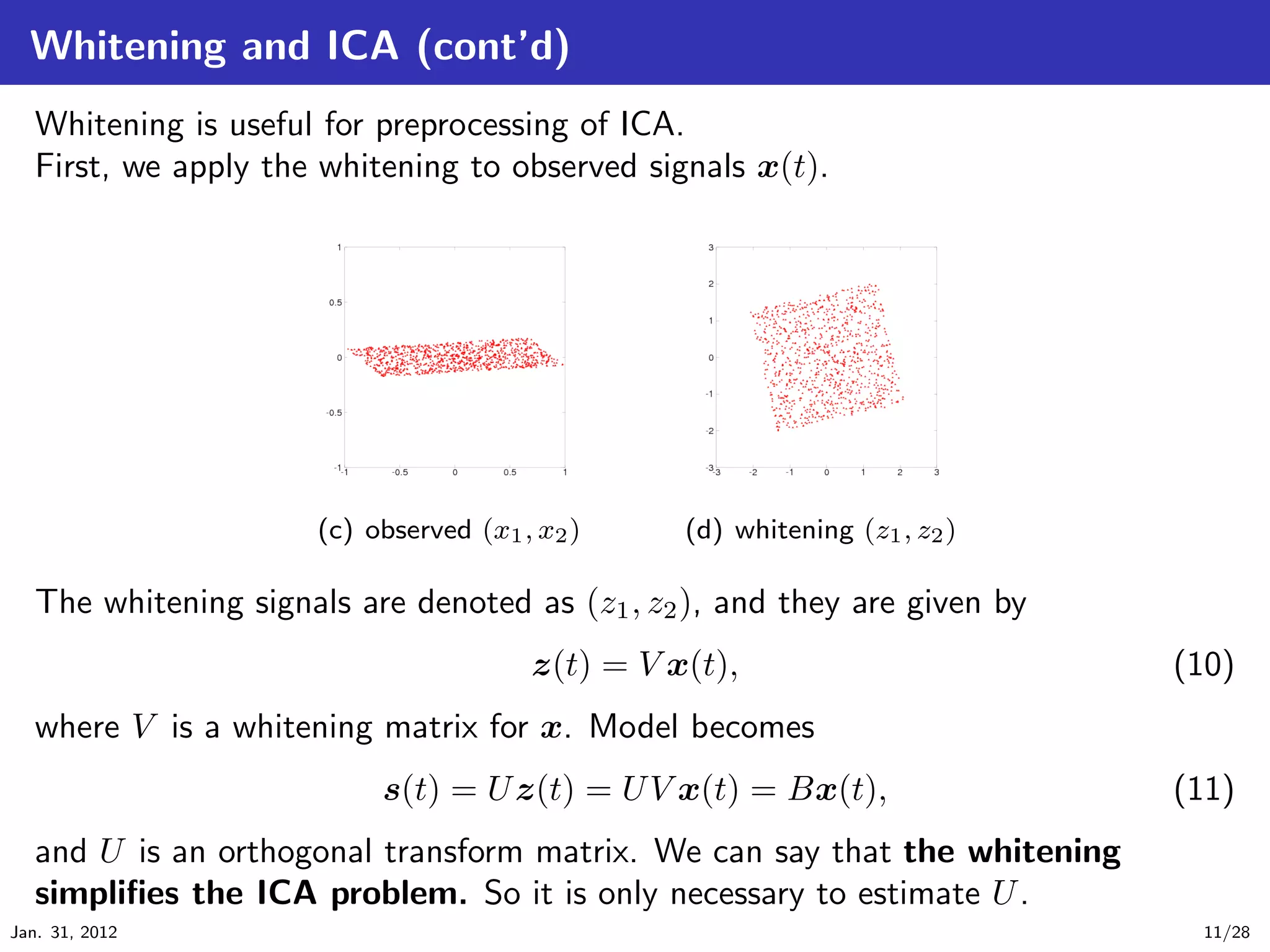
Definition of White signal .
..
White signals are defined as any z which satisfies conditions of
. E[z] = 0, E[zz T ] = I. (9)
.. .
.
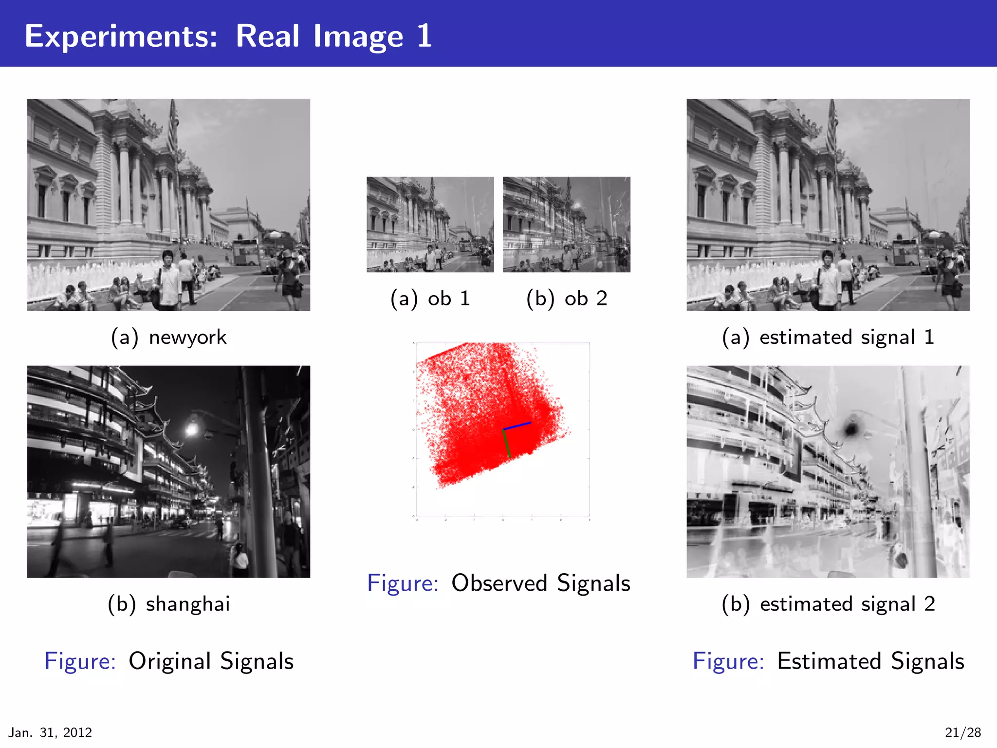
First, we show an example of original independent signals and observed signal as
follow:
(a) source (s1 , s2 ) (b) observed (x1 , x2 )
Observed signals x(t) are given by x(t) = As(t).
ICA give us the original signals s(t) by s(t) = Bx(t).
Jan. 31, 2012 10/28](https://image.slidesharecdn.com/main-120131194743-phpapp02/75/Independent-Component-Analysis-10-2048.jpg)
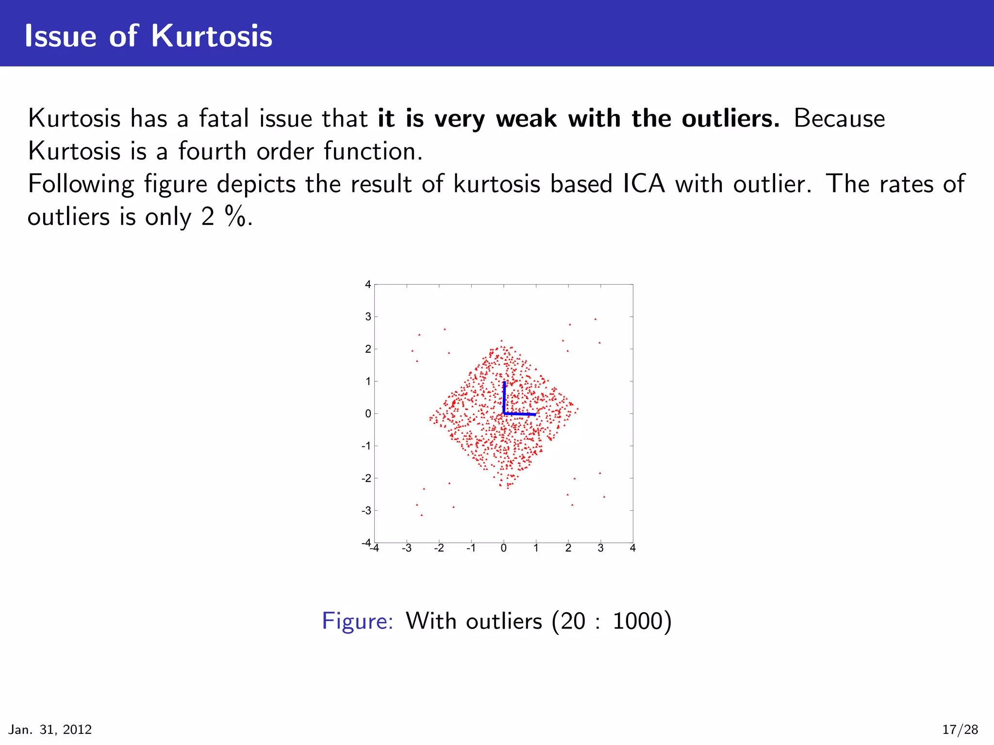
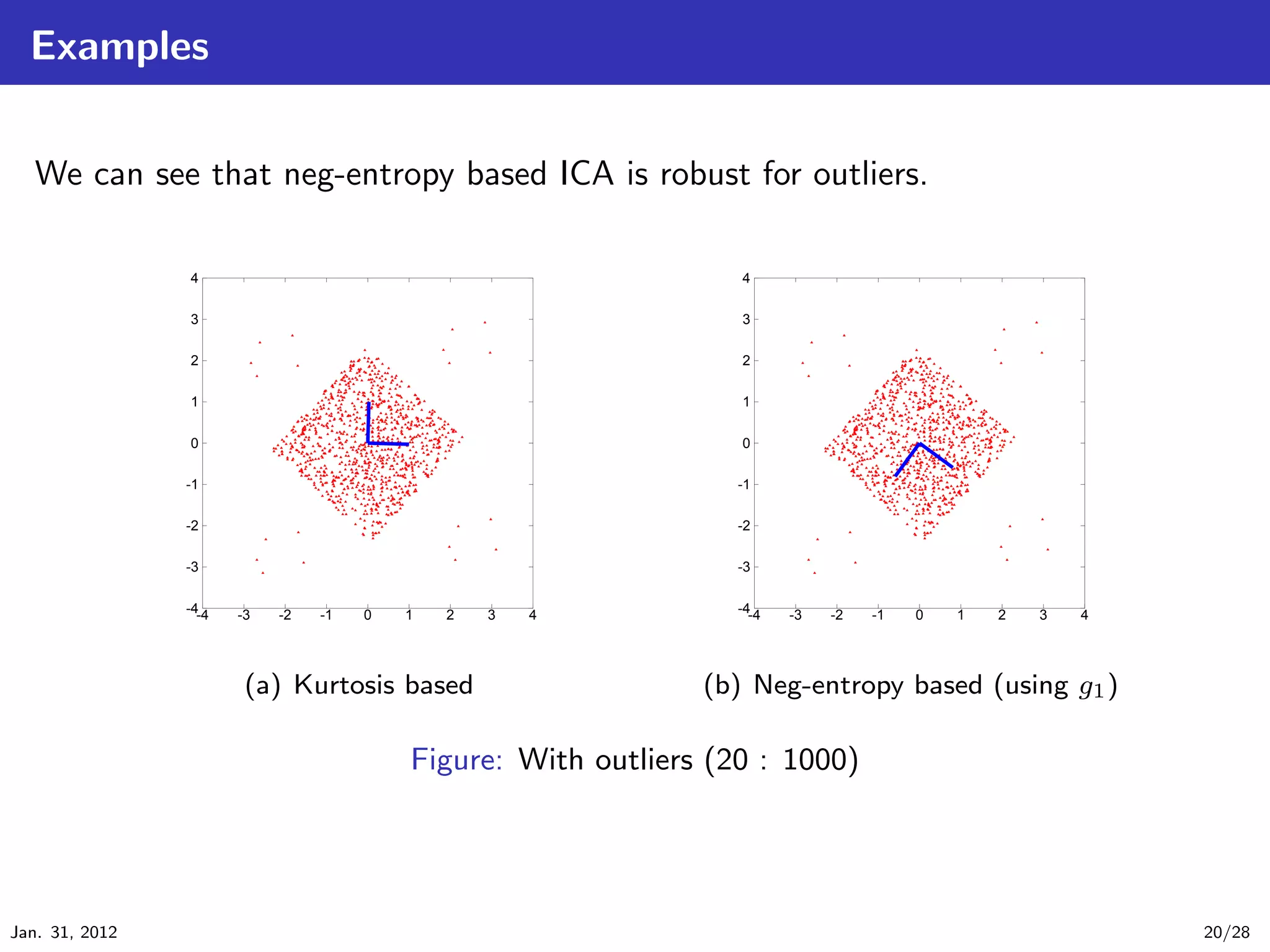
![Maximization of Kurtosis
Kurtosis is a measures of Non-Gaussianity. Kurtosis is defined by
kurt(y) = E[y 4 ] − 3(E[y 2 ])2 . (12)
We assume that y is white (i.e. E[y] = 0, E[y 2 ] = 1 ), then
kurt(y) = E[y 4 ] − 3. (13)
We can solve the ICA problem by
ˆ
b = max |kurt(bT x(t))|. (14)
b
Jan. 31, 2012 13/28](https://image.slidesharecdn.com/main-120131194743-phpapp02/75/Independent-Component-Analysis-13-2048.jpg)
![Fast ICA algorithm based on Kurtosis
We consider z is a white signal given from x. And we consider to maximize the
absolute value of kurtosis as
maximize |kurt(wT z)|, s.t. wT w = 1. (15)
Differential of |kurt(wT z)| is given by
∂|kurt(wT z)| ∂
= E{(wT z)4 } − 3E{(wT z)2 }2 (16)
∂w ∂w
∂
= E{(wT z)4 } − 3{||w||2 }2 (because E(zz T ) = I) (17)
∂w
= 4sign[kurt(wT z)] E{z(wT z)3 } − 3w||w||2 (18)
Jan. 31, 2012 14/28](https://image.slidesharecdn.com/main-120131194743-phpapp02/75/Independent-Component-Analysis-14-2048.jpg)
![Fast ICA algorithm based on Kurtosis (cont’d)
According to the gradient method, we can obtain following algorithm:
.
Gradient algorithm based on Kurtosis .
..
w ← w + ∆w, (19)
w
w← , (20)
||w||
. ∆w ∝ sign[kurt(wT z)] E{z(wT z)3 } − 3w . (21)
.. .
.
We can see that above algorithm converge when w ∝ ∆w. And w and −w are
equivalent solution, so we can obtain another algorithm:
.
Fast ICA algorithm based on Kurtosis .
..
w ← E{z(wT z)3 } − 3w, (22)
w
w← . (23)
. ||w||
.. .
.
It is well known as a fast convergence algorithm for ICA !!
Jan. 31, 2012 15/28](https://image.slidesharecdn.com/main-120131194743-phpapp02/75/Independent-Component-Analysis-15-2048.jpg)
![Fast ICA algorithm based on Neg-entropy
The approximation procedure of neg-entropy is complex, then it is omitted here.
We just introduce the fast ICA algorithm based on neg-entropy:
.
Fast ICA algorithm based on Neg-entropy .
..
w ← E[zg(wT z)] − E[g (wT z)]w (26)
w
w← (27)
. ||w||
.. .
.
where we can select functions g and g from
.
.. g1 (y) = tanh(a1 y) and g1 (y) = a1 (1 − tanh2 (a1 y)),
1
.
.. g2 (y) = y exp(−y 2 /2) and g (y) = (1 − y 2 ) exp(−y 2 /2),
2
2
...
3 g3 (y) = y 3 and g3 (y) = 3y 2 .
1 ≤ a1 ≤ 2.
Please note that (g3 , g3 ) is equivalent to Kurtosis based ICA.
Jan. 31, 2012 19/28](https://image.slidesharecdn.com/main-120131194743-phpapp02/75/Independent-Component-Analysis-19-2048.jpg)
![Approaches of ICA
In this research area, many method for ICA are studied and proposed as follow:
.
.. Criteria of ICA [Hyv¨rinen et al., 2001]
1 a
Non-Gaussianity based ICA*
Kurtosis based ICA*
Neg-entropy based ICA*
MLE based ICA
Mutual information based ICA
Non-linear ICA
Tensor ICA
...
2 Solving Algorithm for ICA
gradient method*
fast fixed-point algorithm* [Hyv¨rinen and Oja, 1997]
a
(‘*’ were introduced today.)
Jan. 31, 2012 25/28](https://image.slidesharecdn.com/main-120131194743-phpapp02/75/Independent-Component-Analysis-25-2048.jpg)
![Summary
I introduced about BSS problem and basic ICA techniques (Kurtosis,
Neg-entropy).
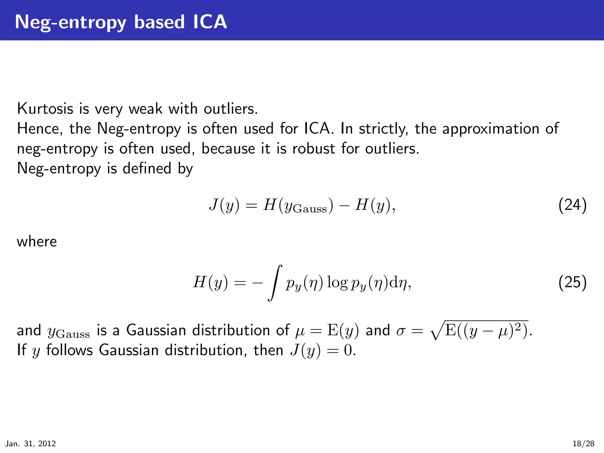
Kurtosis is weak with outliers.
Neg-entropy is proposed as a robust measure of Non-Gaussianity.
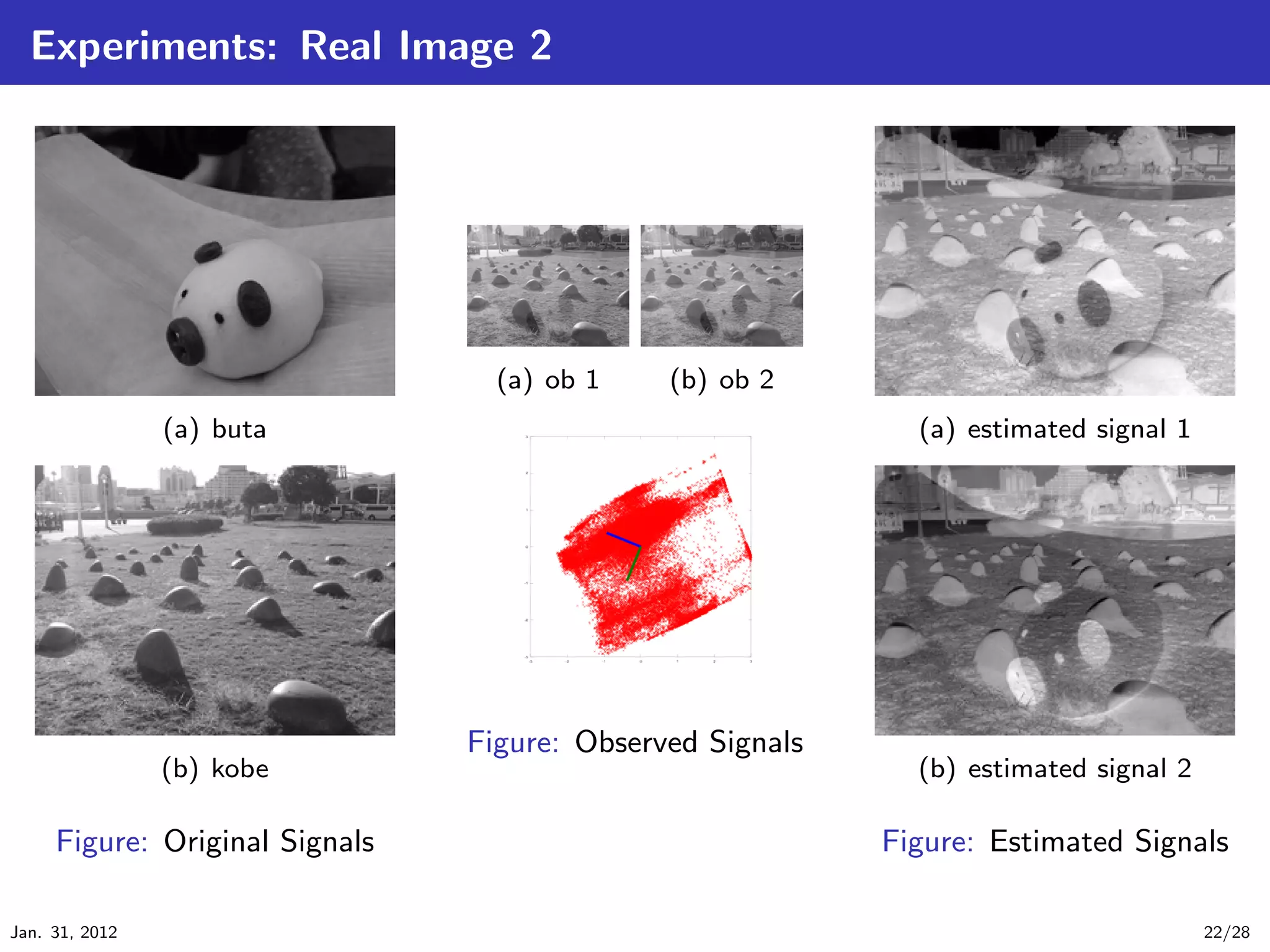
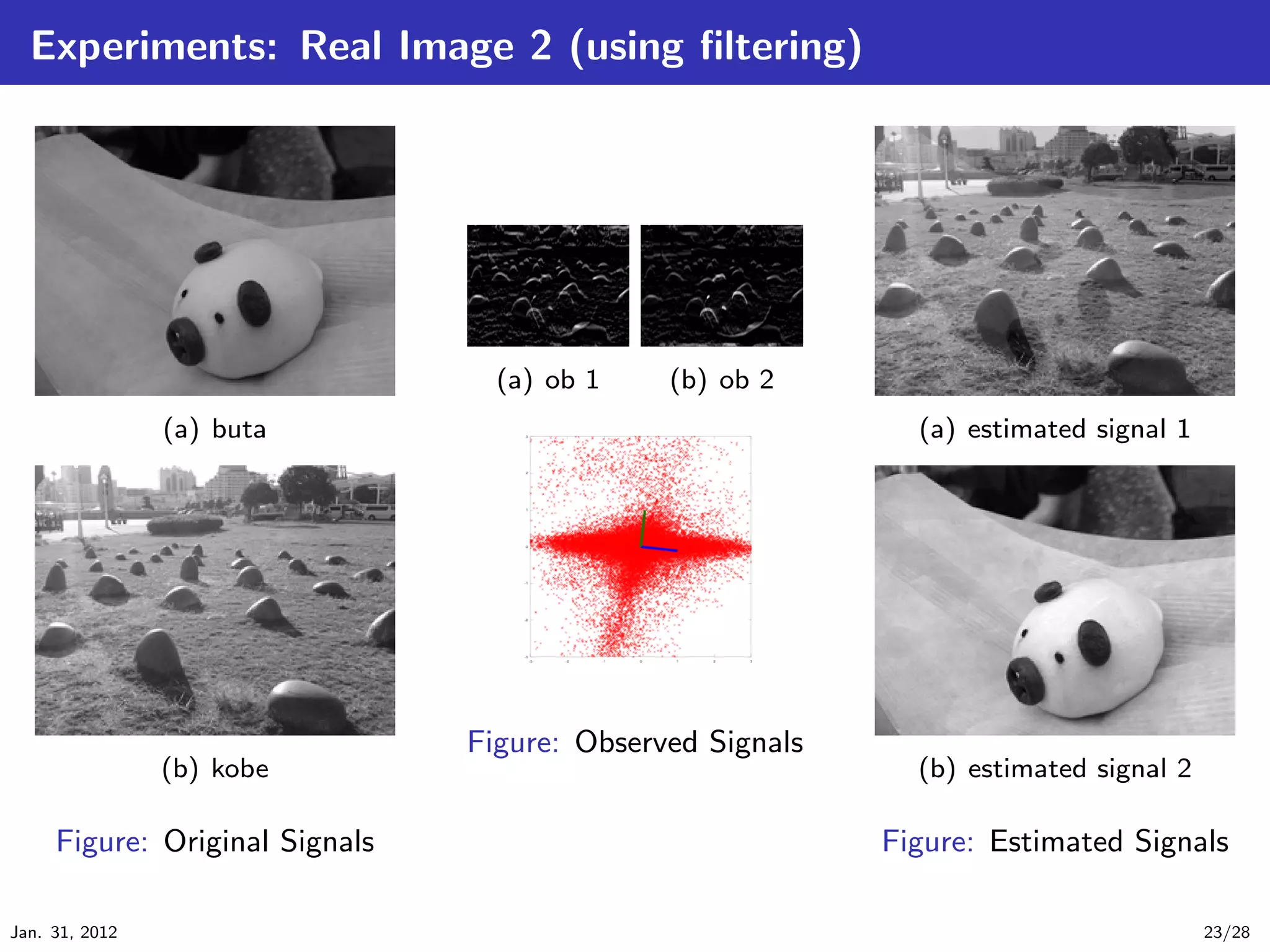
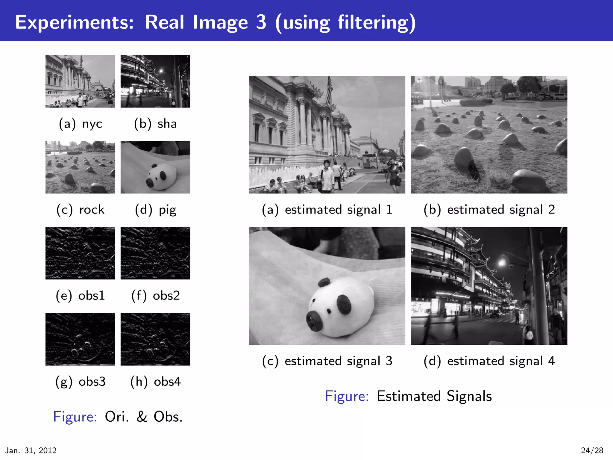
I conducted experiments of ICA using Image data.
In some case, worse results are obtained.
But I solved this issue by using differential filter.
This technique is proposed in [Hyv¨rinen, 1998].
a
We knew that the differential filter is very effective for ICA.
Jan. 31, 2012 26/28](https://image.slidesharecdn.com/main-120131194743-phpapp02/75/Independent-Component-Analysis-26-2048.jpg)
![Bibliography I
[Hyv¨rinen, 1998] Hyv¨rinen, A. (1998).
a a
Independent component analysis for time-dependent stochastic processes.
[Hyv¨rinen et al., 2001] Hyv¨rinen, A., Karhunen, J., and Oja, E. (2001).
a a
Independent Component Analysis.
Wiley.
[Hyv¨rinen and Oja, 1997] Hyv¨rinen, A. and Oja, E. (1997).
a a
A fast fixed-point algorithm for independent component analysis.
Neural Computation, 9:1483–1492.
Jan. 31, 2012 27/28](https://image.slidesharecdn.com/main-120131194743-phpapp02/75/Independent-Component-Analysis-27-2048.jpg)


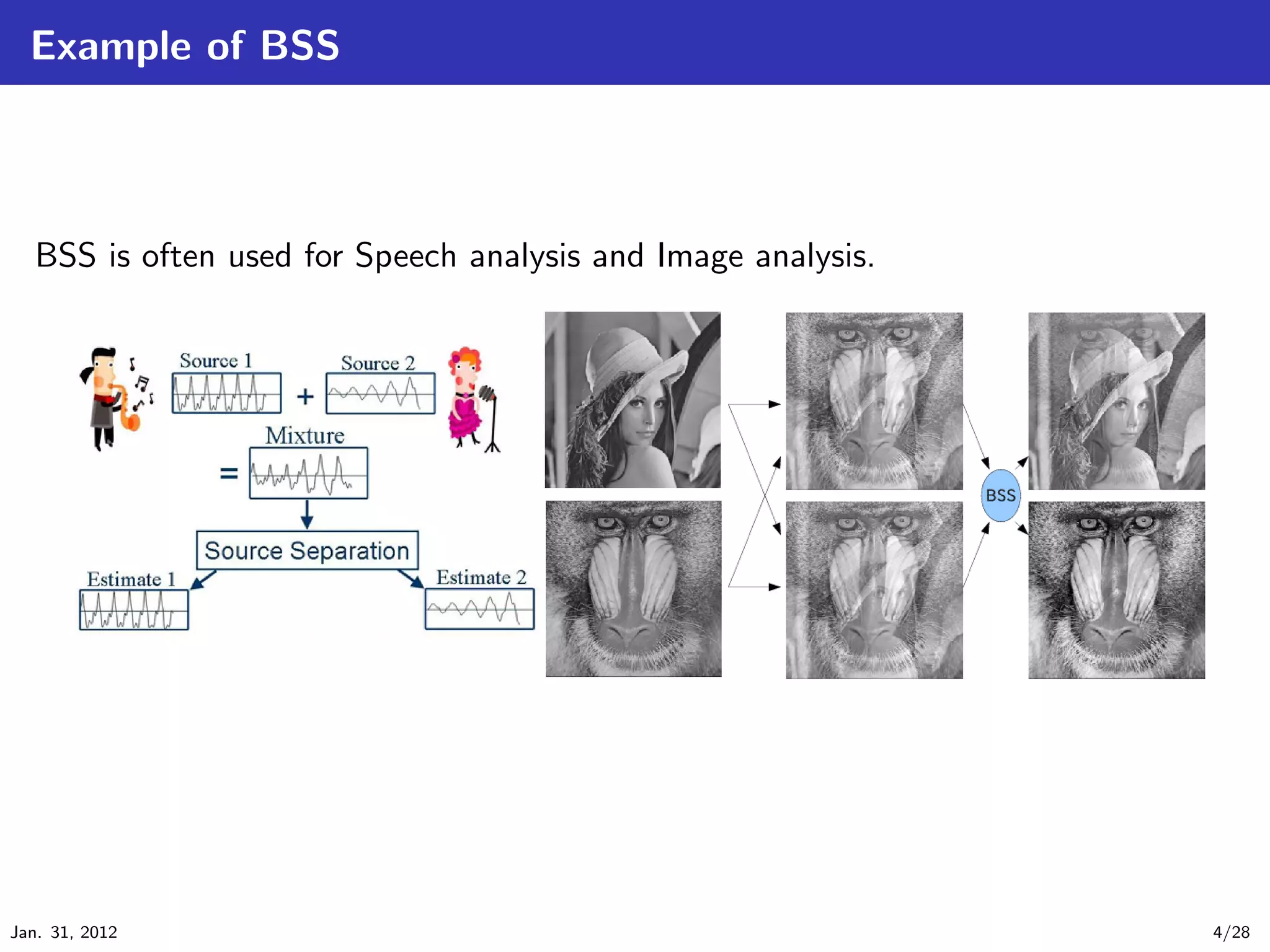
This document discusses independent component analysis (ICA) for blind source separation. ICA is a method to estimate original signals from observed signals consisting of mixed original signals and noise. It introduces the ICA model and approach, including whitening, maximizing non-Gaussianity using kurtosis and negentropy, and fast ICA algorithms. The document provides examples applying ICA to separate images and discusses approaches to improve ICA, including using differential filtering. ICA is an important technique for blind source separation and independent component estimation from observed signals.


![Ica group 3[1]](https://cdn.slidesharecdn.com/ss_thumbnails/icagroup31-191026172214-thumbnail.jpg?width=640&height=640&fit=bounds)


![Coded Agents – with UiPath SDK + LangGraph [Virtual Hands-on Workshop]](https://cdn.slidesharecdn.com/ss_thumbnails/codedagentsdeck-251215155422-5497c599-thumbnail.jpg?width=640&height=640&fit=bounds)


