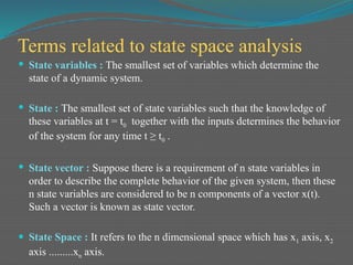
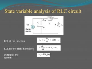
The document discusses state variable analysis as a method to analyze dynamic circuits and obtain their transfer functions using matrix notations and Laplace transformations. It covers the application of state variables in various systems, including mechanical, thermodynamic, electronic, and ecological systems, and elaborates on concepts like state space, state variables, and their relationships with controllability and observability in control systems. It also includes MATLAB code examples for modeling state-space representations of systems.

1. STATE VARIABLE ANALYSIS
By
Suvro Kundu
M.E., Microwave
Roll No. : 08
Burdwan University

2. Introduction
 A way of analyzing the dynamic circuits in order to obtain its transfer
function.
 Uses Matrix notations and Laplace transformations.
 It can be applied to non linear system.
 It can be applied to tile invariant systems.
 It can be applied to multiple input multiple output systems.
 Its gives idea about the internal state of the system.

3. Uses of State Variable
 In mechanical systems, the position coordinates and velocities of
mechanical parts are typical state variables.
 In thermodynamics, a state variable is also called a state function.
Examples include temperature, pressure, volume, internal energy,,
and entropy.
 In electronic circuits, the voltages of the nodes and
the currents through components in the circuit are usually the state
variables.
 In ecosystem model, population sizes (or concentrations) of plants,
animals and resources (nutrients, organic material) are typical state
variables.
 In control engineering and other areas of science and engineering,
state variables are used to represent the states of a general system.

4. State Variables of a Dynamic System

5. Terms related to state space analysis
 State variables : The smallest set of variables which determine the
state of a dynamic system.
 State : The smallest set of state variables such that the knowledge of
these variables at t = t0 together with the inputs determines the behavior
of the system for any time t ≥ t0 .
 State vector : Suppose there is a requirement of n state variables in
order to describe the complete behavior of the given system, then these
n state variables are considered to be n components of a vector x(t).
Such a vector is known as state vector.
 State Space : It refers to the n dimensional space which has x1 axis, x2
axis .........xn axis.

6. State variable analysis of RLC circuit
KCL at the junction
KVL for the right hand loop
Output of the
system

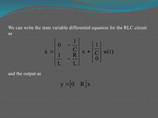
7. We can write the equations as a set of two first order differential
equations in terms of the state variables x1 [vC(t)] and x2 [iL(t)] as
follows:
2
1
2
2
1
x
L
R
x
L
1
dt
dx
)
t
(
u
C
1
x
C
1
dt
dx





L
c
i
)
t
(
u
dt
dv
C 

c
L
L
v
i
R
dt
di
L 


The output signal is then 2
0
1 x
R
)
t
(
v
)
t
(
y 

Utilizing the first-order differential equations and the initial
conditions of the network represented by [x1(t0) x2(t0)], we can
determine the system’s future and its output.

8. )
t
(
u
0
C
1
x
L
R
L
1
C
1
0
x























We can write the state variable differential equation for the RLC circuit
as
and the output as
 x
R
0
y 

9. Bu
Ax
x 


Du
Cx
y 

x

x
y
u
A
B
C
D
= state vector
= derivative of the state vector with respect to
time
= output vector
= input or control vector
= system matrix
= input matrix
= output matrix
= Feed forward
matrix
State equation
Output equation
General State Space of Physical System

10. Correlation between state variable and
transfer functions models

11. Analysis of state variable using matlab
State-space object
Du
Cx
y
Bu
Ax
x





sys=ss(A,B,C,D)
Du
Cx
y
Bu
Ax
x




 )
s
(
U
)
s
(
G
)
s
(
Y 
sys_ss=ss(sys_tf)
sys_tf=tf(sys_ss)
)
s
(
U
)
s
(
G
)
s
(
Y 
Du
Cx
y
Bu
Ax
x





The ss function
sys_tf represents a transfer function model
sys_ss is a state space representation.

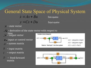
12. For instance, consider the third-order system
6
s
16
s
8
s
6
s
8
s
2
)
s
(
R
)
s
(
Y
)
s
(
G 2
3
2







We can obtain a state-space representation using the ss function. The
state-space representation of the system given by G(s) is
num=[2 8 6];den=[1 8 16 6];
sys_tf=tf(num,den)
sys_ss=ss(sys_tf)
Matlab code
   
0
D
and
75
.
0
1
1
C
0
0
2
B
,
0
1
0
0
0
4
5
.
1
4
8
A






















 




13. For the system Bu
Ax
x 


we can determine whether the system is controllable by examining the
algebraic condition
  n
B
A
B
A
AB
B
rank 1
n
2



The matrix A is an nxn matrix an B is an nx1 matrix. For multi input systems, B can
be nxm, where m is the number of inputs.
For a single-input, single-output system, the controllability matrix Pc is
described in terms of A and B as
 
B
A
B
A
AB
B
P 1
n
2
c

 
which is nxn matrix. Therefore, if the determinant of Pc is nonzero, the
system is controllable.
A system is completely controllable if there exists an unconstrained control u(t) that can
transfer any initial state x(t0) to any other desired location x(t) in a finite time, t0≤t≤T.
Controllability

14. Observability
A system is completely observable if and only if there exists a finite time T
such that the initial state x(0) can be determined from the
observation history y(t) given the control u(t).
Cx
y
and
Bu
Ax
x 



Consider the single-input, single-output system
where C is a 1xn row vector, and x is an nx1 column vector. This system is
completely observable when the determinant of the observability matrix P0 is
nonzero.













 1
n
O
A
C
A
C
C
P

The det P0=1, and the system is completely observable.

15. Conclusion
 Enables us to describe the nth order system.
 The stability, controllability and observability of
the network can be determined easily.
 The solution of first order differential equation is
comparatively easier.

16. Thank You