I have made these slides. Get help if it could.

1. CALCULUS
EARLYTRANSCEDENTIALS BY HAVARD ANTON

2. CONTENT:
Chapter 2: Limits and Derivatives
2.2: The Limit Of a Function

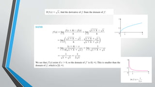
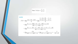
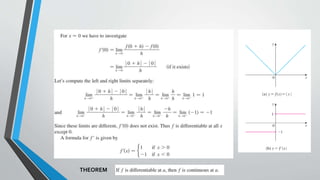
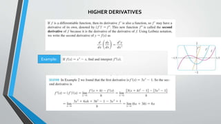
3. LIMITS
Limits are a fundamental concept in calculus that describe the
behavior of a function as its input (or argument) approaches a certain
value.
• They help us understand the value that a function approaches as
the input gets closer and closer to a given point, even if the
function doesn't actually reach that value at the point.
• This concept is crucial for dealing with situations where direct
evaluation of a function at a point is difficult or impossible, such as
points of discontinuity or where the function tends toward infinity.

4. For Instance:
Begin by considering a simple function,
such as:
and what happens as x approaches 2.
SOL: Numerator would become zero.
Hence: We can't evaluate the function
directly at x=2.
By the way…..
What if zero is
divided by any
number???

5. 2
0
F(x)
x

6. TANGENT LINESAND LIMITS
A line is called tangent to a circle if it meets the circle at precisely one point
Although this definition is adequate for circles, it is not appropriate for more general curves.
To obtain a definition of a tangent line that applies to curves other than circles,
we must view tangent lines another way. For this purpose, suppose that we are
interested in the tangent line at a point P on a curve in the xy-plane and that Q
is any point that lies on the curve and is different from P. The line through P and
Q is called a secant line for the curve at P. Intuition suggests that if we move the
point Q along the curve toward P, then the secant line will rotate toward a
limiting position. The line in this limiting position is what we will consider to be
the tangent line at P

9. AREAS AND LIMITS
For plane regions with straight-line boundaries, areas can
often be calculated by subdividing the region into rectangles
or triangles and adding the areas of the constituent parts
However, for regions with curved boundaries, such as that in
Figure 1.7- a more general approach is needed. One such
approach is to begin by approximating the area of the region
by inscribing a number of rectangles of equal width under the
curve and adding the areas of these rectangles

10. DECIMALS AND LIMITS

11. LIMITS:
The most basic use of limits is to describe how a function
behaves as the independent variable approaches a given value.
Let us examine the behavior of the function:
for x-values closer and closer to 2. It is evident from the graph and table in Figure 1.1.8 that the values
of f (x) get closer and closer to 3 as values of x are selected closer and closer to 2 on either the left or
the right side of 2. We describe this by saying that the “limit of x2 − x + 1 is 3 as x approaches 2 from
either side,” and we write:

13. Try this!!!!!!

14. SOLUTION:
Notice that the function is not defined when ,but that doesn’t matter because the
definition of says that we consider values of x that are close to a but not equal to a .
The tables give values of f(x) (correct to six decimal places) for values of that approach 1 (but are not equal
to 1). On the basis of the values in the tables, we make the guess that

15. Now let’s change f slightly by giving it the value 2 when x=1 and calling the resulting function :
This new function g still has the same limit as x approaches 1 (fig 2)

16. The table lists values of the function for several values of near 0.
As t approaches 0, the values of the function seem to approach
0.166666 and so we guess that

17. The function is not defined when
From the table at the left and the graph in Figure we guess that

18. DIY

19. ONE-SIDED LIMITS

20. The graph of a function g is shown in Figure. Use it to state the values (if they exist) of the following:

22. As x approaches 0, the values of f (x) = |x|/x approach −1 from
the left and approach 1 from the right.Thus, the one-sided
limits at 0 are not the same.

23. Try this!!!!!!

25. INFINITE LIMITS
Sometimes one-sided or two-sided limits fail to exist because
the values of the function increase or decrease without bound
Consider the behavior of f (x) = 1/x for values of x near 0. It is evident from the table
and graph in Figure 1.1.15 that as x-values are taken closer and closer to 0 from the
right, the values of f (x) = 1/x are positive and increase without bound; and as x-
values are taken closer and closer to 0 from the left, the values of f (x) = 1/x are
negative and decrease without bound. We describe these limiting behaviors by
writing
The symbols + and − here
are not real numbers; they
simply describe particular
ways in which the limits
fail to exist. Do not make
the mistake of
manipulating these
symbols using rules of
algebra. For example, it is
incorrect to write (+) − (+)
= 0.

28. VERTICAL ASYMPTOTES
Figure 1.1.17 illustrates geometrically what happens when any
of the following situations occur:
In each case the graph of y = f (x) either rises or falls without bound, squeezing closer
and closer to the vertical line x = a as x approaches a from the side indicated in the limit.
The line x = a is called a vertical asymptote of the curve y = f (x) (from the Greek word
asymptotos, meaning “nonintersecting”).

29. DIY

30. COMPUTING LIMITS
• First we will obtain the limits of some simple functions.
• Then we will develop a repertoire of theorems that will enable us to use the limits of those simple
functions as building blocks for finding limits of more complicated functions.

31. Contd…
The following theorem will be our basic tool for finding limits algebraically.

32. This theorem can be stated informally as follows:
(a)The limit of a sum is the sum of the limits.
(b)The limit of a difference is the difference of the limits.
(c)The limit of a product is the product of the limits.
(d )The limit of a quotient is the quotient of the limits, provided the limit of
the denominator is not zero.
(e)The limit of an nth root is the nth root of the limit.
A constant factor can be moved through a limit symbol.

33. Question: Solution:
Question: Solution:
Question: Solution:

34. If we use the Product Law repeatedly with g(x)=f(x) , we obtain the following law
In applying these six limit laws, we need to use two special limits:
If we now put f(x)=x in Law 6 and use Law 8, we get another useful special limit
A similar limit holds for roots as follows.

35. Try this!!!!!!
Evaluate the following limits and justify each step

36. A constant can be moved
through a limit symbol.

37. Recall that a rational function is a ratio of two polynomials.
Theorem 1.2.2(d )
Theorem 1.2.3

38. In all three parts the limit of the numerator is −2, and the limit of the denominator is 0,
so the limit of the ratio does not exist.To be more specific than this, we need to analyze
the sign of the ratio.The sign of the ratio, which is given in Figure 1.2.3, is
determined by the signs of 2 − x, x − 4, and x + 2.

39. From the right, the ratio is always negative; and as x
approaches 4 from the left, the ratio is eventually positive.
Thus,
Because the one-sided limits have opposite signs, all we can
say about the two-sided limit
is that it does not exist.

40. Solve this as your homework:
We can’t apply the Quotient Law immediately, since the limit of the denominator
is 0. Here the preliminary algebra consists of rationalizing the numerator:

41. Some limits are best calculated by first finding the left- and right-hand limits.
The next two theorems give two additional properties of limits
The Squeeze Theorem, which is
sometimes called the Sandwich
Theorem or the Pinching Theorem. It
says that if g(x) is squeezed between
f(x) and h(x) near a, and if f and h have
the same limit L at a, then g is forced
to have the same limit L at a.

43. A Function Can be in Pieces​​ We can create functions that behave
differently based on the input (x) value. A function made up of 3 pieces.
LIMITS OF PIECEWISE-DEFINED FUNCTIONS
We will determine the stated two-sided limit by first considering the corresponding one-sided limits. For
each one-sided limit, we must use that part of the formula that is applicable on the interval over which x
varies. For example, as x approaches −2 from the left, the applicable part of the formula is
and as x approaches −2 from the right, the applicable part of the formula near −2 is

44. Thus,
from which it follows that lim x→−2f (x) does not exist.

46. DIY

47. 2.5 Continuity
A function f is continuous at a number a if
The definition says that f is continuous at a if f(x) approaches f(a) as xapproaches a.Thus a
continuous function f has the property that a small change in xproduces only a small change in
f(X) . In fact,the change in f(x) can be kept as small as we please by keeping the change in x
sufficiently small.

48. Where are each of the following functions discontinuous?
a) Notice that f(2) is not defined,so f is discontinuous at 2. Later we’ll see why f is continuous at all
other numbers.
does not exist. So, f is discontinuous at 0.

50. Theorem-A function f is continuous from the right at a number a if
and is continuous from the left at a if
Theorem-A function f is continuous on an interval if it is continuous at every number in the
interval. (If f is defined only on one side of an endpoint of the interval, we understand
continuous at the endpoint to mean continuous from the right or continuous from the left.)

53. The Derivatives As a Function
we considered the derivative of a function fat a fixed number a:
Here we change our point of view and let the number avary. If we replace a in Equation1 by a
variable x,we obtain
Given any number x for which this limit exists, we assign to x the number . So we can regard as
a new function, called the derivative of f.

55. a) When using Equation 2 to compute a derivative, we must remember that the variable is
and that is temporarily regarded as a constant during the calculation of the limit.
b)We use a graphing device to graph and in Figure 3. Notice that when has horizontal tangents
and is positive when the tangents have positive slope. So these graphs serve as a check on our
work in part (a).

59. If we use y=f(x) the traditional notation to indicate that the independent variable is and the
dependent variable is ,then some common alternative notations for the derivative are as
follows
The symbols D and d/dx are called differentiation operators because they indicate
the operation of differentiation, which is the process of calculating a derivative.

61. THEOREM

62. HOW CAN A FUNCTION FAILTO BE DIFFERENTIABLE?
In general, if the graph of a function has a “corner”or “kink”in it, then the graph of f has no
tangent at this point and f is not differentiable there.
If is not continuous at , then is not differentiable at . So at any discontinuity (for instance, a
jump discontinuity) fails to be differentiable
1.
2.
3. A third possibility is that the curve has a vertical tangent line when x=a; that is f, is
continuous at a and
This means that the tangent lines become steeper and steeper
as x approaches a .

64. HIGHER DERIVATIVES
Example:

65. For n-th derivative
DIY