1
4
Límites y
Derivadas
2
Límites y la Derivada
• Límites
• Límites Laterales
• Continuidad
• La Derivada
3
Introducción al Cálculo
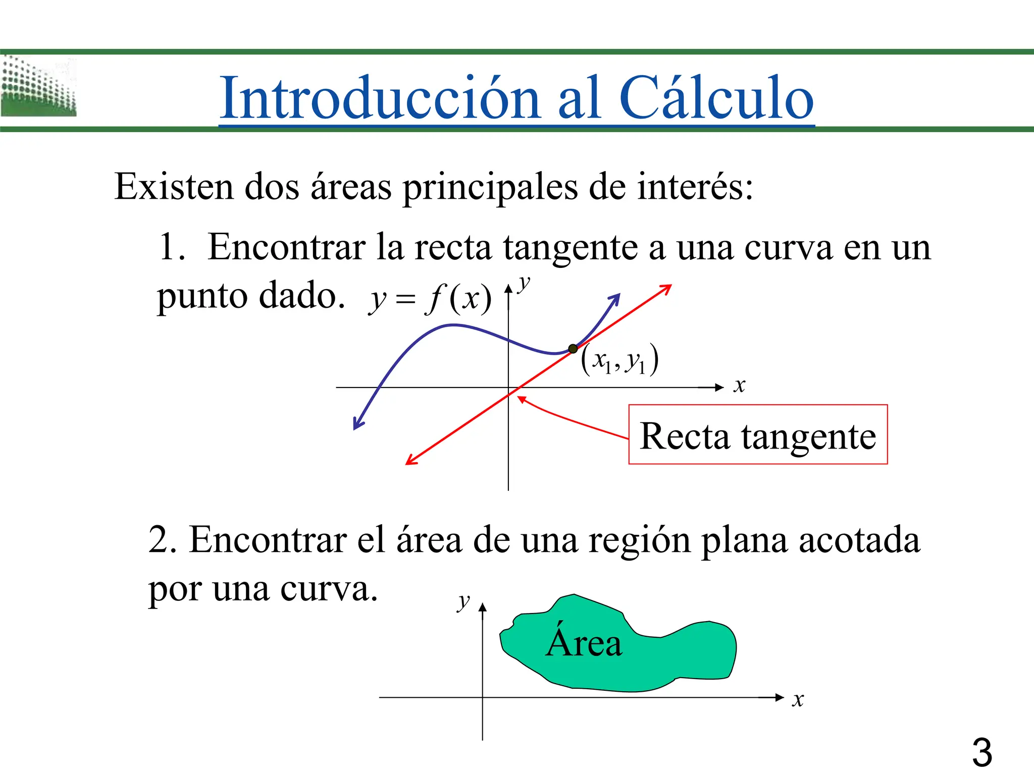
Existen dos áreas principales de interés:
1. Encontrar la recta tangente a una curva en un
punto dado. ( )
y f x

Recta tangente
 
1 1
,
x y
2. Encontrar el área de una región plana acotada
por una curva.
Área
x
x
y
y
4
Velocidad
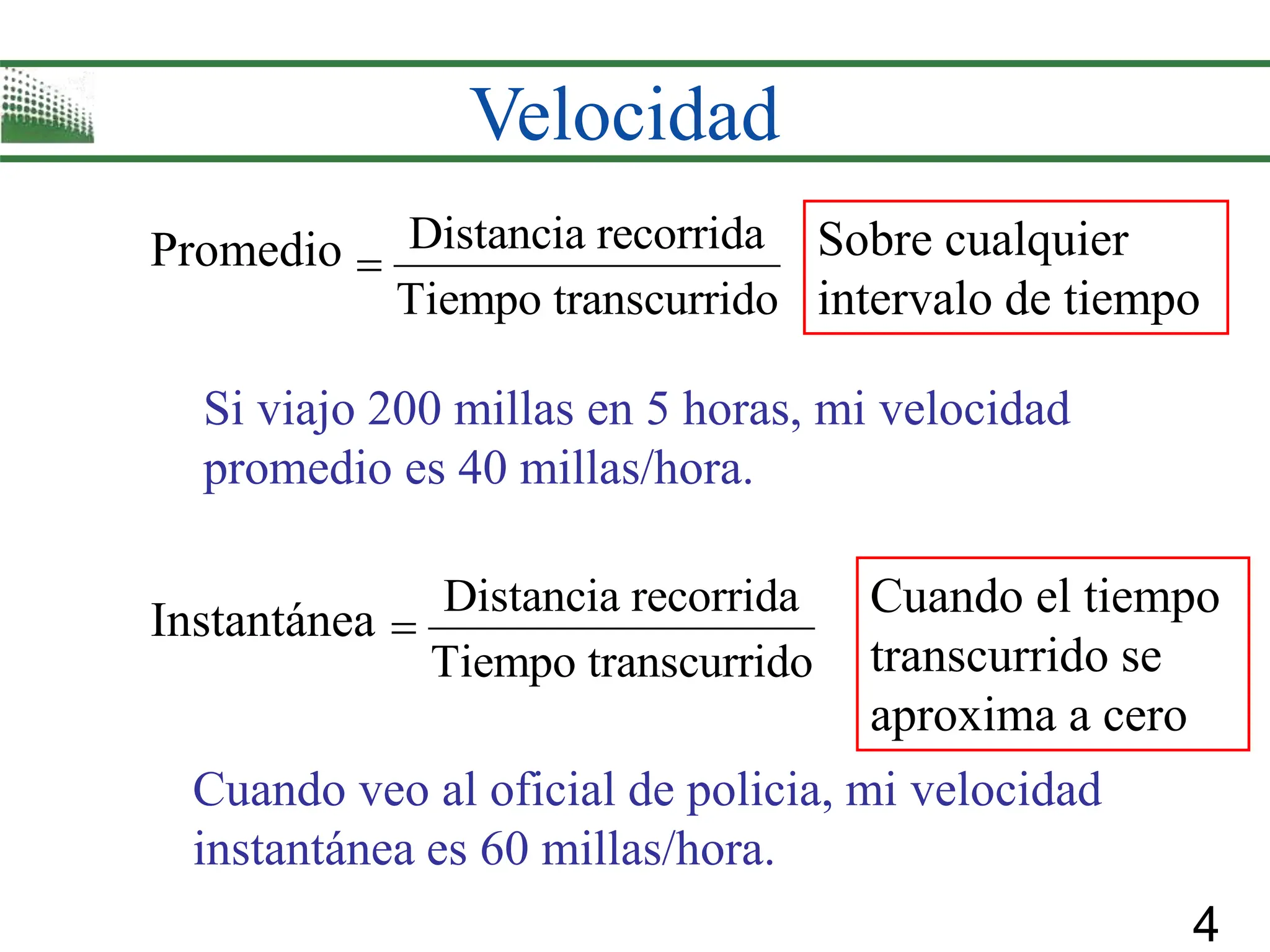
Promedio Distancia recorrida
Tiempo transcurrido

Instantánea Cuando el tiempo
transcurrido se
aproxima a cero
Sobre cualquier
intervalo de tiempo
Si viajo 200 millas en 5 horas, mi velocidad
promedio es 40 millas/hora.
Cuando veo al oficial de policia, mi velocidad
instantánea es 60 millas/hora.
Distancia recorrida
Tiempo transcurrido

5
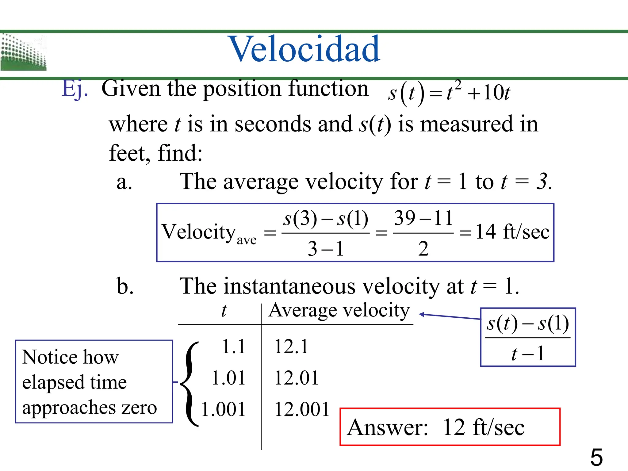
Velocidad
Ej. Given the position function   2
10
s t t t
 
where t is in seconds and s(t) is measured in
feet, find:
a. The average velocity for t = 1 to t = 3.
b. The instantaneous velocity at t = 1.
ave
(3) (1) 39 11
Velocity 14 ft/sec
3 1 2
s s
 
  

Average velocity
t
( ) (1)
1
s t s
t


1.1 12.1
1.001 12.001
1.01 12.01
Answer: 12 ft/sec

Notice how
elapsed time
approaches zero
6
Límite de una Funcción
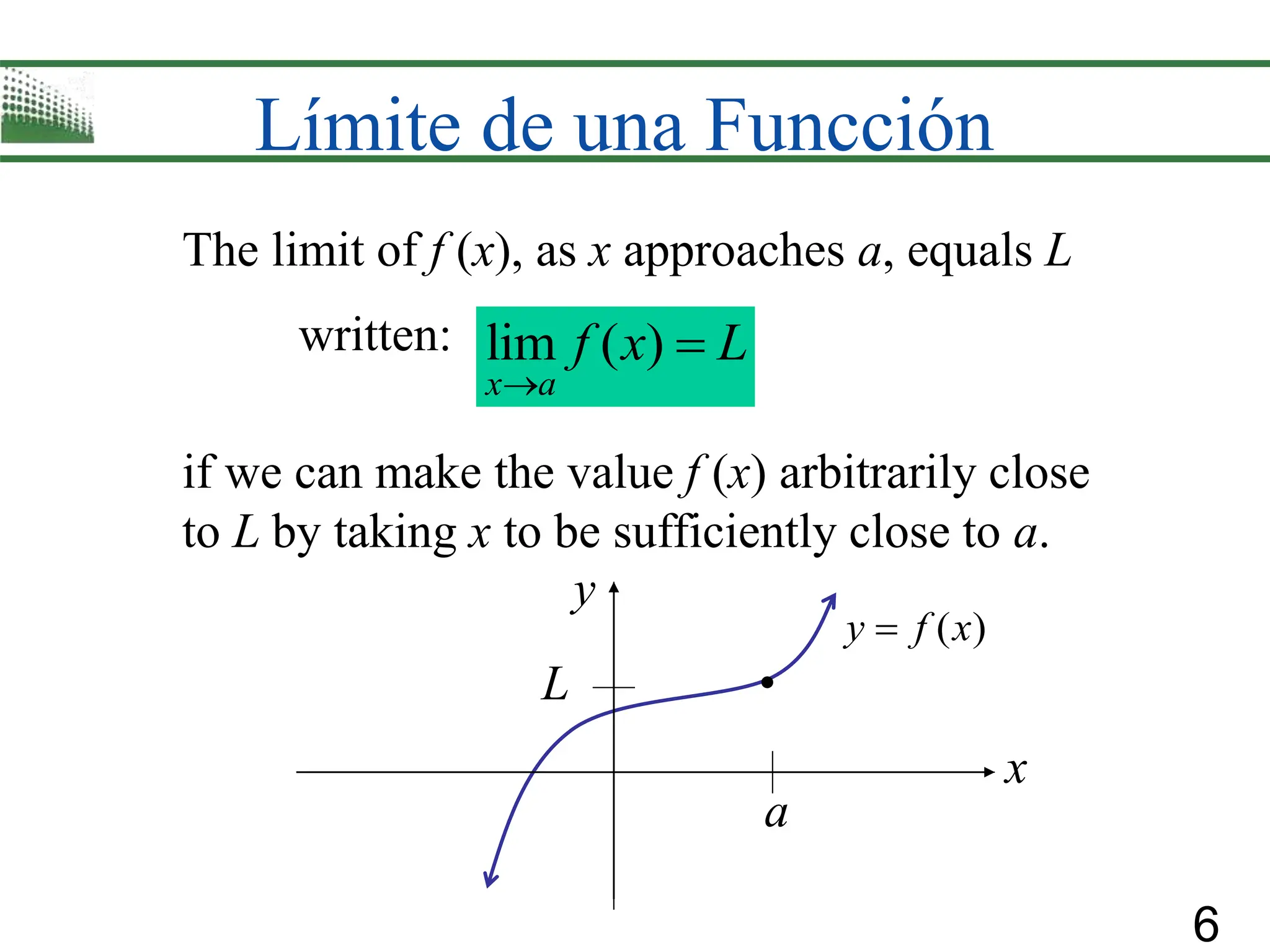
The limit of f (x), as x approaches a, equals L
written:
if we can make the value f (x) arbitrarily close
to L by taking x to be sufficiently close to a.
lim ( )
x a
f x L


a
L
( )
y f x

x
y
7
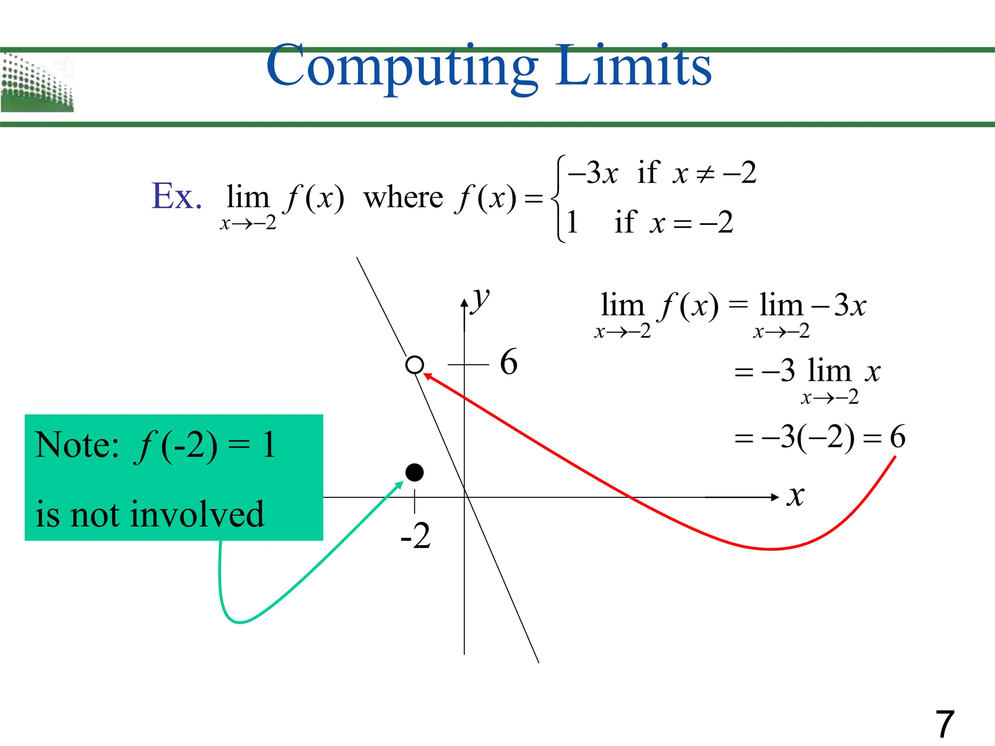
Computing Limits
Ex.
2
3 if 2
lim ( ) where ( )
1 if 2
x
x x
f x f x
x

  

 
 

6
-2
2 2
lim ( ) = lim 3
x x
f x x
 

2
3 lim
3( 2) 6
x
x

 
   
Note: f (-2) = 1
is not involved
x
y
8
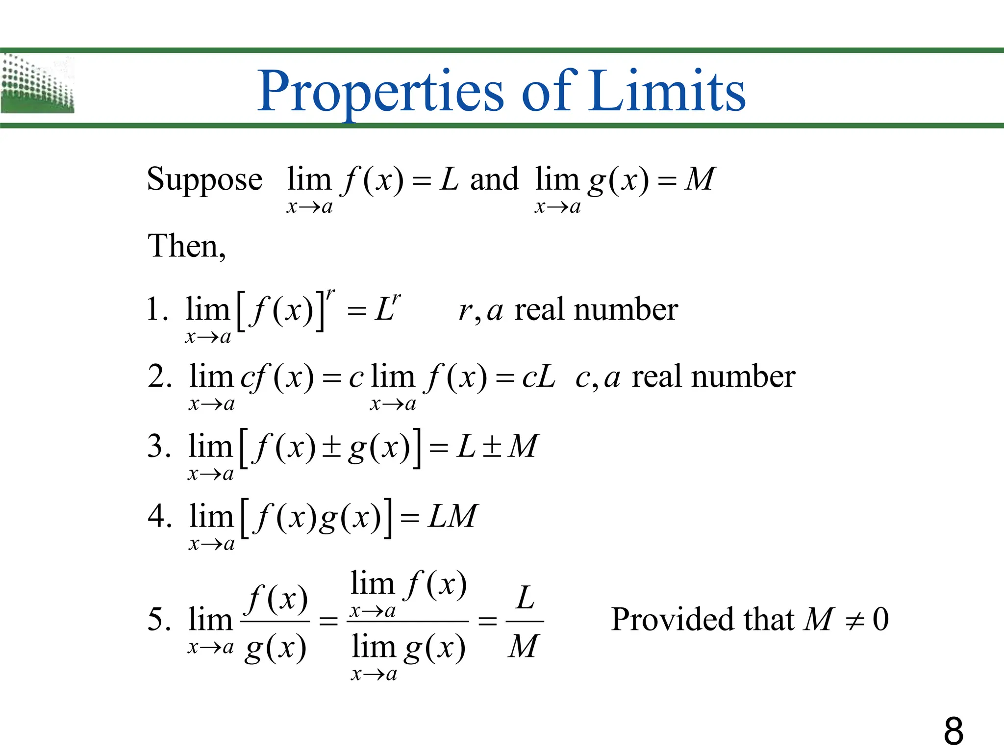
Properties of Limits
 
 
 
Suppose lim ( ) and lim ( )
Then,
1. lim ( ) , real number
2. lim ( ) lim ( ) , real number
3. lim ( ) ( )
4. lim ( ) ( )
lim ( )
( )
5. lim
( ) lim
x a x a
r r
x a
x a x a
x a
x a
x a
x a
f x L g x M
f x L r a
cf x c f x cL c a
f x g x L M
f x g x LM
f x
f x
g x
 

 




 

 
  

 Provided that 0
( )
x a
L
M
g x M

 
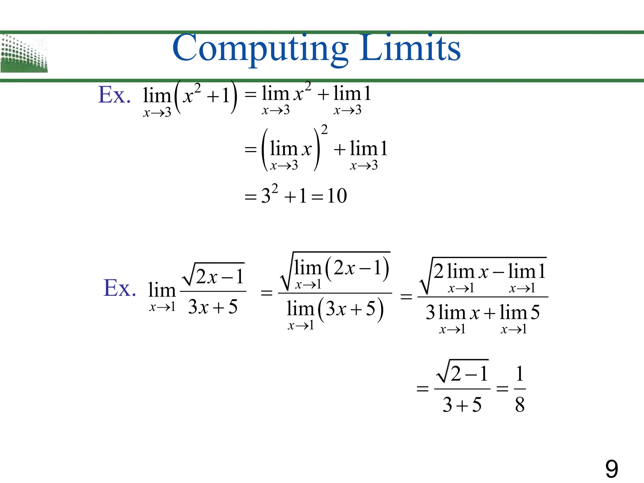
9
Computing Limits
Ex.
Ex.
 
2
3
lim 1
x
x


2
3 3
lim lim1
x x
x
 
 
 
2
3 3
2
lim lim1
3 1 10
x x
x
 
 
  
1
2 1
lim
3 5
x
x
x



 
 
1
1
lim 2 1
lim 3 5
x
x
x
x





1 1
1 1
2lim lim1
3lim lim5
x x
x x
x
x
 
 



2 1 1
3 5 8

 

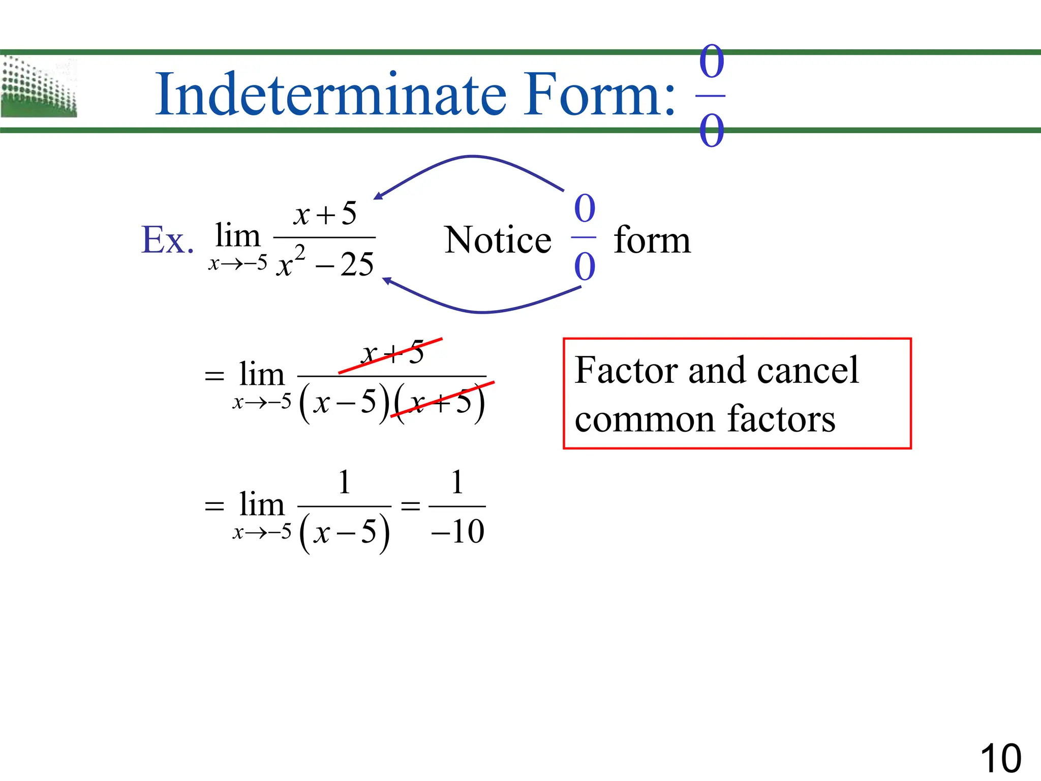
10
Indeterminate Form:
0
0
2
5
5
lim
25
x
x
x



Ex. Notice form
0
0
  
5
5
lim
5 5
x
x
x x



 
 
5
1 1
lim
5 10
x x

 
 
Factor and cancel
common factors
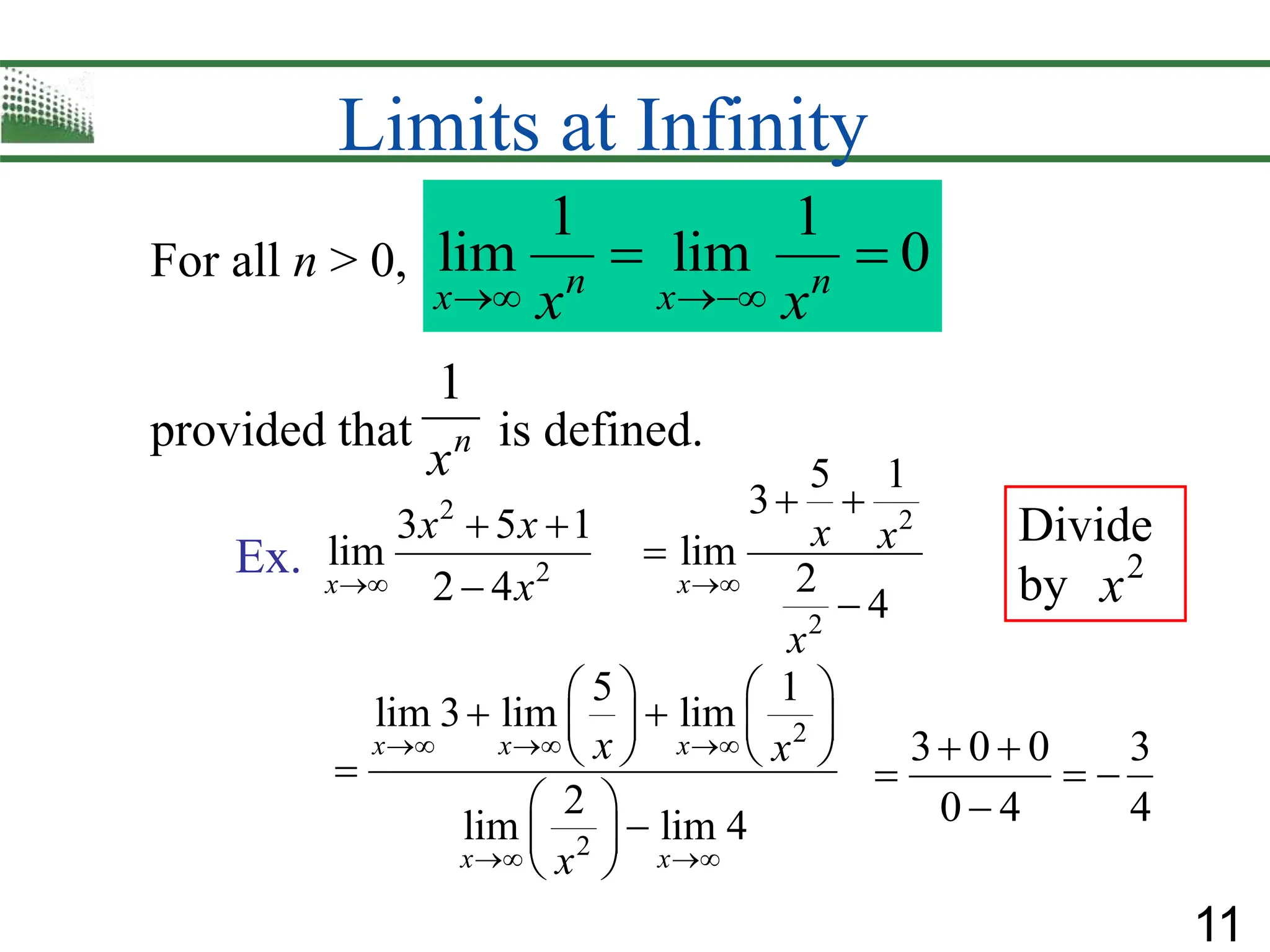
11
Limits at Infinity
For all n > 0,
1 1
lim lim 0
n n
x x
x x
 
 
provided that is defined.
1
n
x
Ex.
2
2
3 5 1
lim
2 4
x
x x
x

 

2
2
5 1
3
lim
2
4
x
x x
x

 


3 0 0 3
0 4 4
 
  

Divide
by 2
x
2
2
5 1
lim 3 lim lim
2
lim lim 4
x x x
x x
x x
x
  
 
   
 
   
   

 

 
 
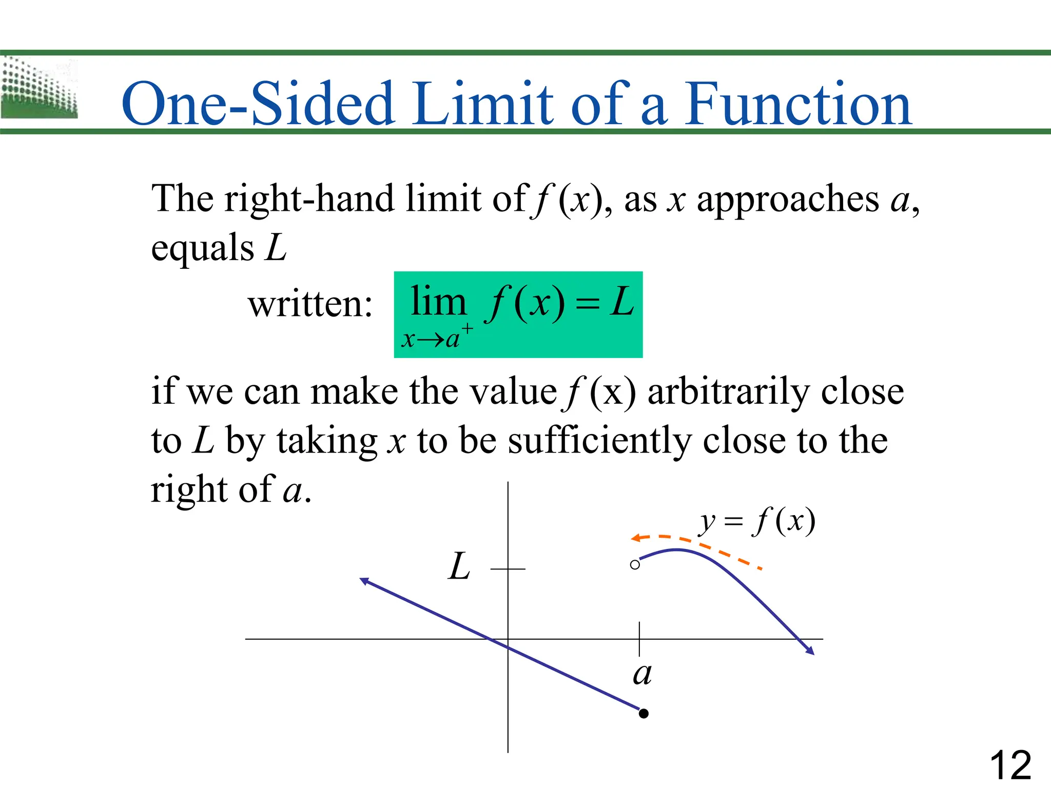
12
One-Sided Limit of a Function
The right-hand limit of f (x), as x approaches a,
equals L
written:
if we can make the value f (x) arbitrarily close
to L by taking x to be sufficiently close to the
right of a.
lim ( )
x a
f x L



a
L
( )
y f x

13
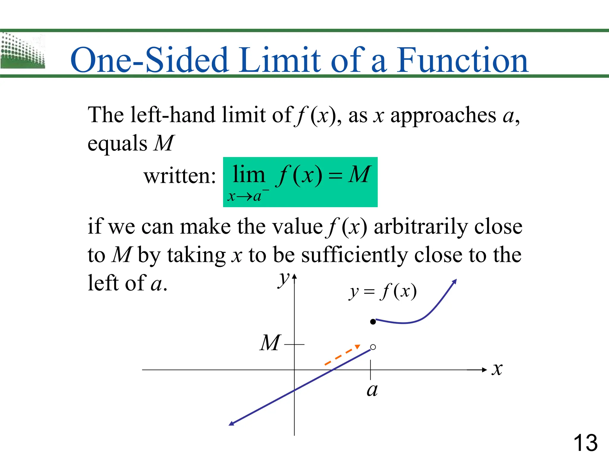
One-Sided Limit of a Function
The left-hand limit of f (x), as x approaches a,
equals M
written:
if we can make the value f (x) arbitrarily close
to M by taking x to be sufficiently close to the
left of a.
lim ( )
x a
f x M



a
M
( )
y f x

x
y
14
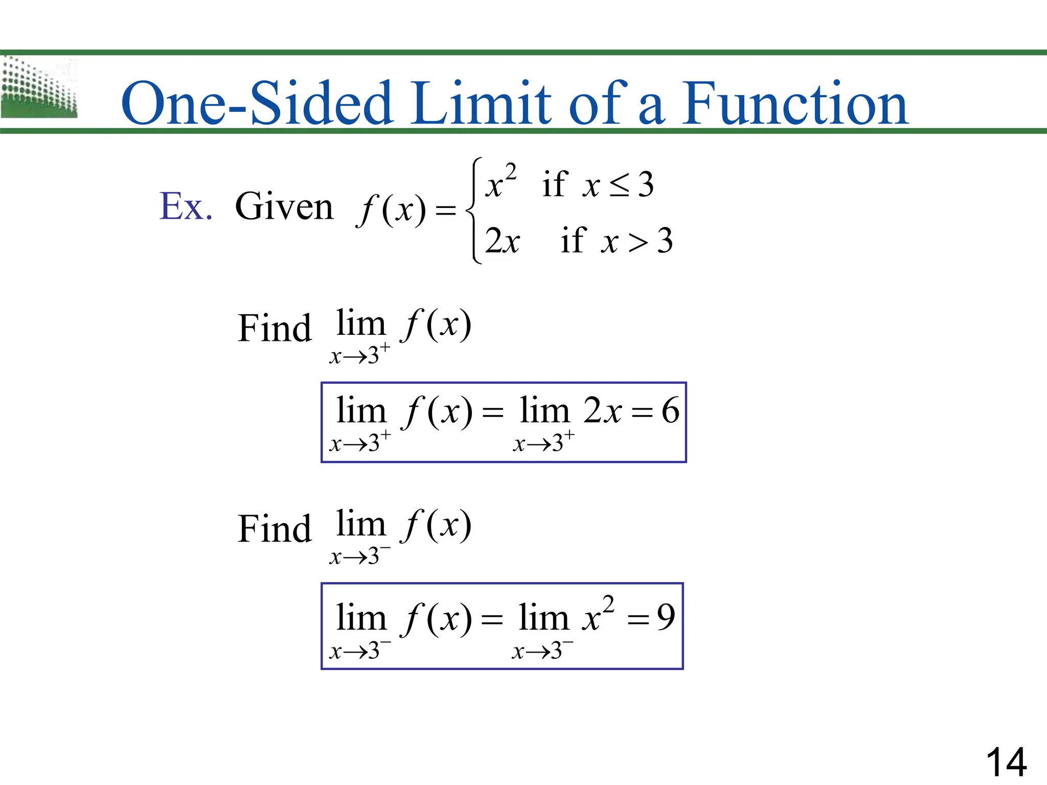
One-Sided Limit of a Function
2
if 3
( )
2 if 3
x x
f x
x x
 

 



Ex. Given
3
lim ( )
x
f x


3 3
lim ( ) lim 2 6
x x
f x x
 
 
 
2
3 3
lim ( ) lim 9
x x
f x x
 
 
 
Find
Find
3
lim ( )
x
f x


15
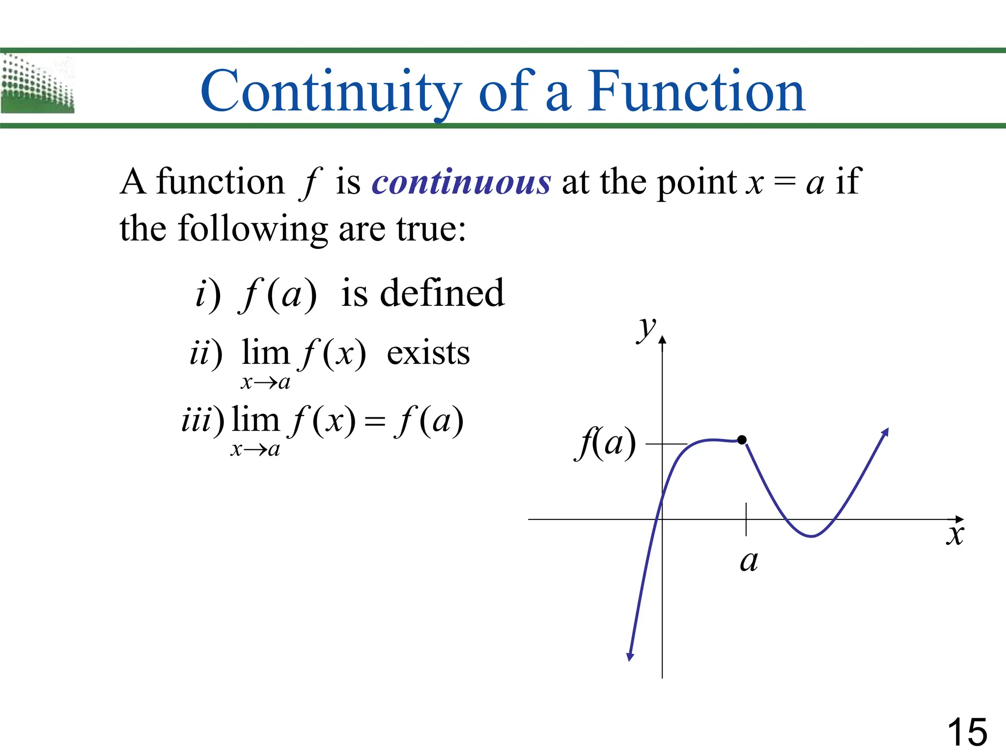
Continuity of a Function
A function f is continuous at the point x = a if
the following are true:
) ( ) is defined
i f a
) lim ( ) exists
x a
ii f x

)lim ( ) ( )
x a
iii f x f a


a
f(a)
y
x
16
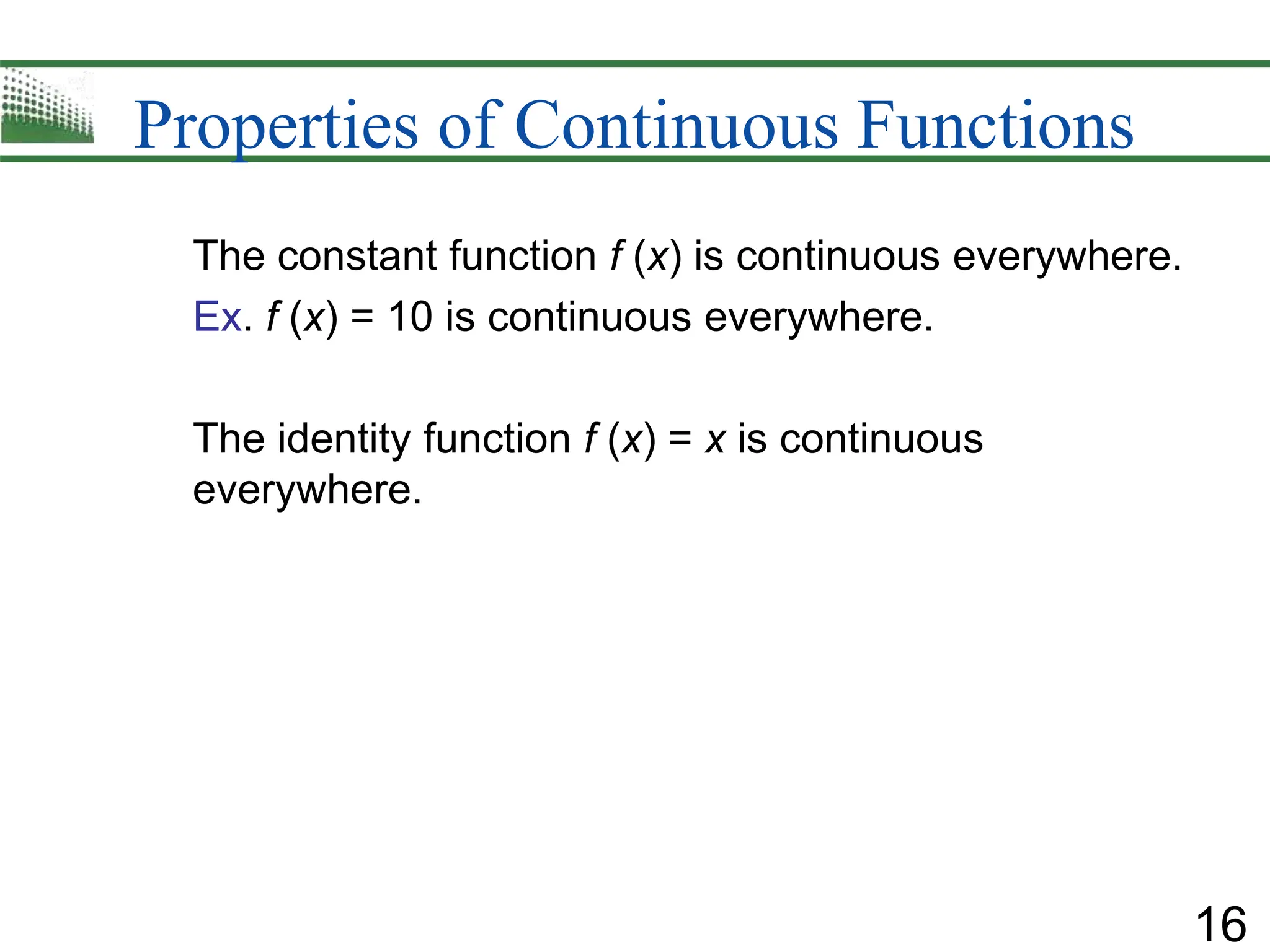
Properties of Continuous Functions
The constant function f (x) is continuous everywhere.
Ex. f (x) = 10 is continuous everywhere.
The identity function f (x) = x is continuous
everywhere.
17
Properties of Continuous Functions
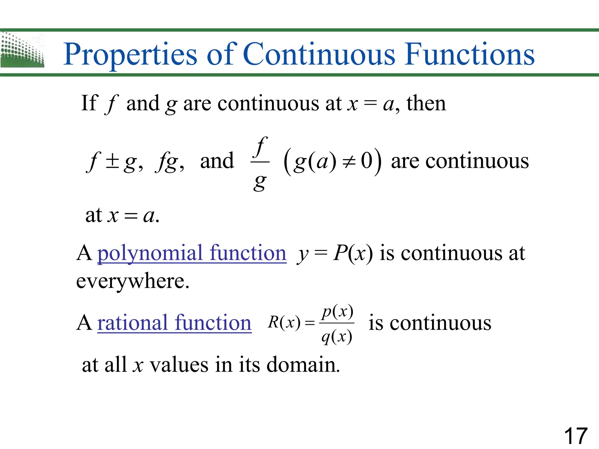
A polynomial function y = P(x) is continuous at
everywhere.
A rational function is continuous
at all x values in its domain.
( )
( )
( )
p x
R x
q x

If f and g are continuous at x = a, then
 
, , and ( ) 0 are continuous
at .
f
f g fg g a
g
x a
 

18
Intermediate Value Theorem
If f is a continuous function on a closed interval [a, b]
and L is any number between f (a) and f (b), then there
is at least one number c in [a, b] such that f(c) = L.
( )
y f x

a b
f (a)
f (b)
L
c
f (c) =
x
y
19
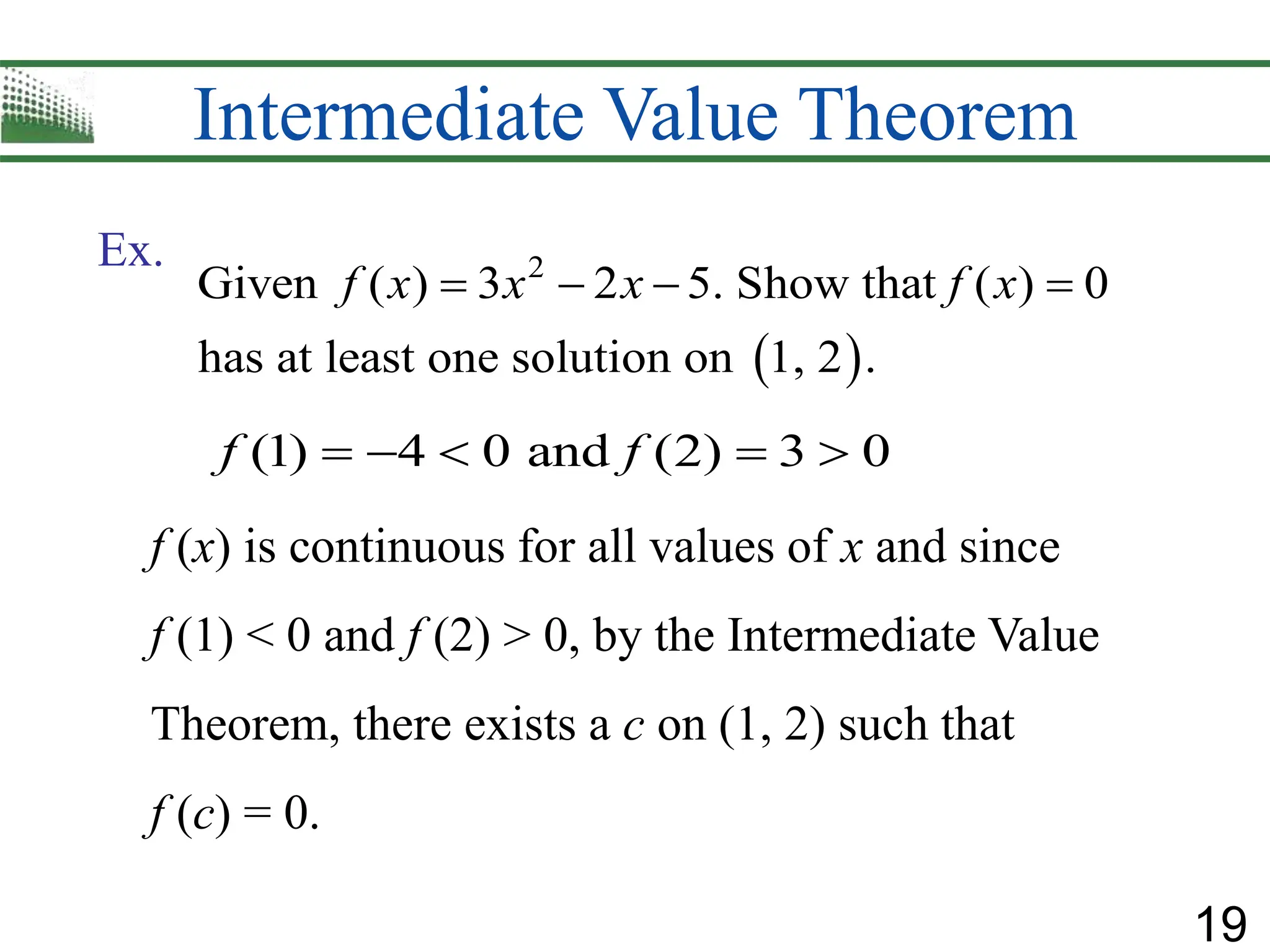
Intermediate Value Theorem
 
2
Given ( ) 3 2 5. Show that ( ) 0
has at least one solution on 1, 2 .
f x x x f x
   
Ex.
(1) 4 0 and (2) 3 0
f f
    
f (x) is continuous for all values of x and since
f (1) < 0 and f (2) > 0, by the Intermediate Value
Theorem, there exists a c on (1, 2) such that
f (c) = 0.
20
Existence of Zeros of a Continuous
Function
If f is a continuous function on a closed interval [a, b],
and f(a) and f(b) have opposite signs, then there is at least
one solution of the equation f(x) = 0 in the interval (a, b).
f(b)
f(a)
a
b
x
y
21
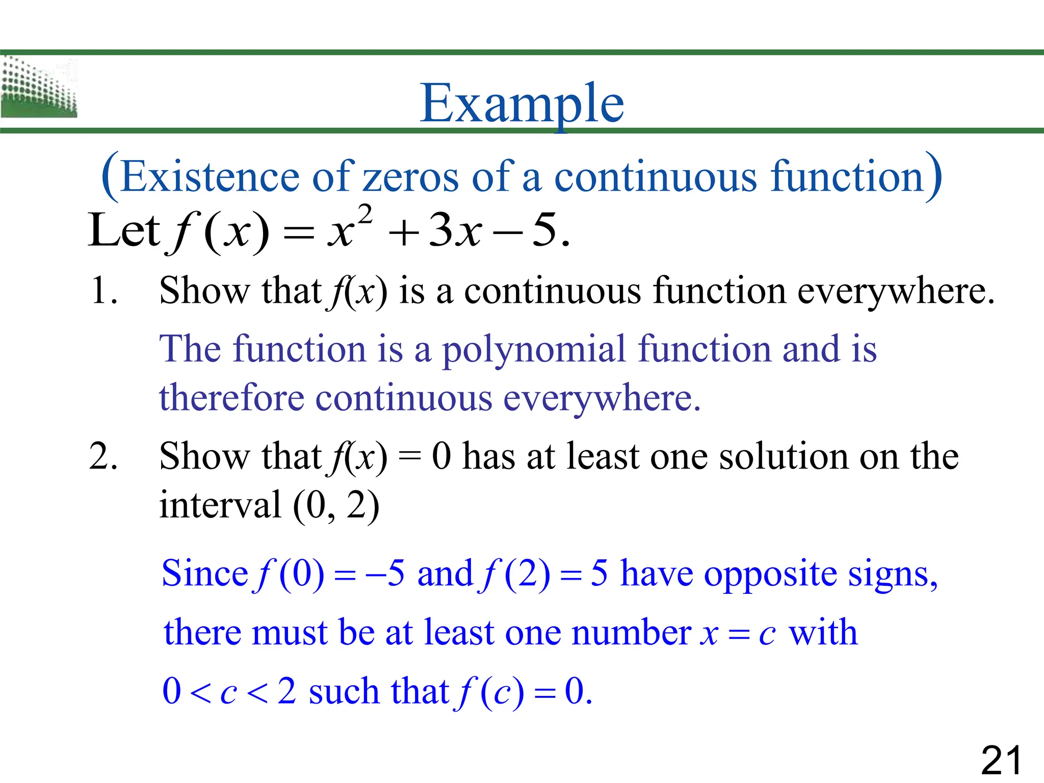
Example
(Existence of zeros of a continuous function)
1. Show that f(x) is a continuous function everywhere.
The function is a polynomial function and is
therefore continuous everywhere.
2. Show that f(x) = 0 has at least one solution on the
interval (0, 2)
Since (0) 5 and (2) 5 have opposite signs,
there must be at least one number with
0 2 such that ( ) 0.
f f
x c
c f c
  

  
2
Let ( ) 3 5.
f x x x
  
22
Rates of Change
Average rate of change of f over the interval
[x, x+h]
( ) ( )
f x h f x
h
 

Instantaneous rate of change of f at x
Slope of the
Tangent Line
Slope of Secant Line
0
( ) ( )
lim
h
f x h f x
h

 

23
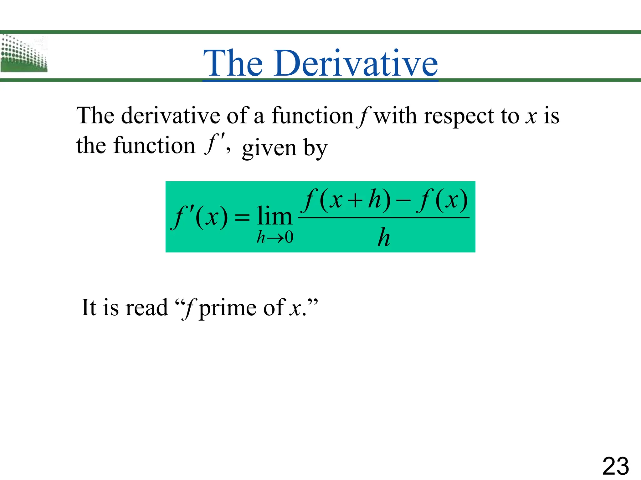
The Derivative
0
( ) ( )
( ) lim
h
f x h f x
f x
h

 
 
The derivative of a function f with respect to x is
the function ,
f  given by
It is read “f prime of x.”
24
The Derivative
0
( ) ( )
( ) lim
h
f x h f x
f x
h

 
 
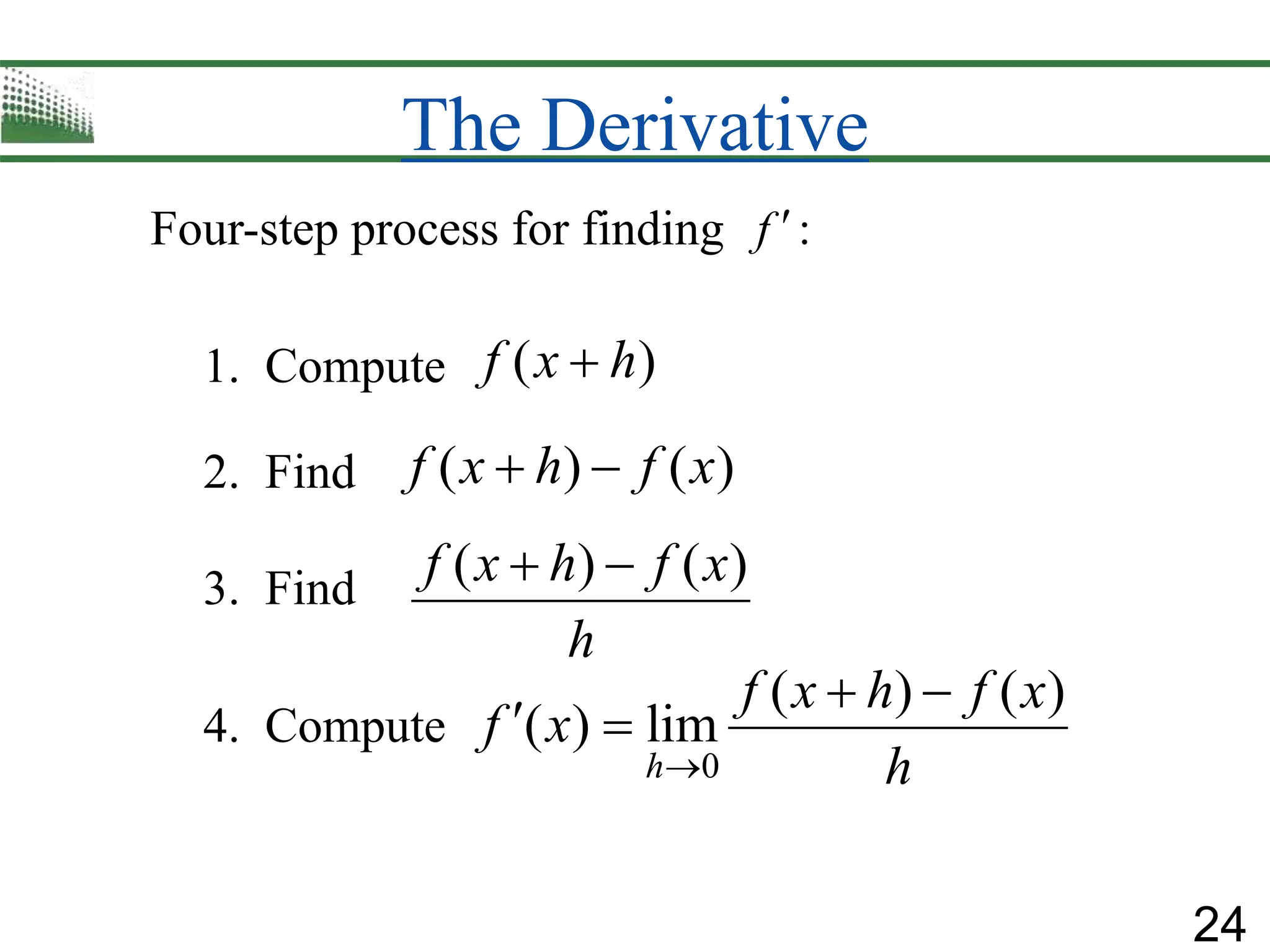
Four-step process for finding :
f 
( ) ( )
f x h f x
 
( ) ( )
f x h f x
h
 
( )
f x h

1. Compute
2. Find
3. Find
4. Compute
25
The Derivative
 
2
0 0
0
( ) ( ) 4 2
lim lim
lim 4 2 4
h h
h
f x h f x xh h
h h
x h x
 

  

   
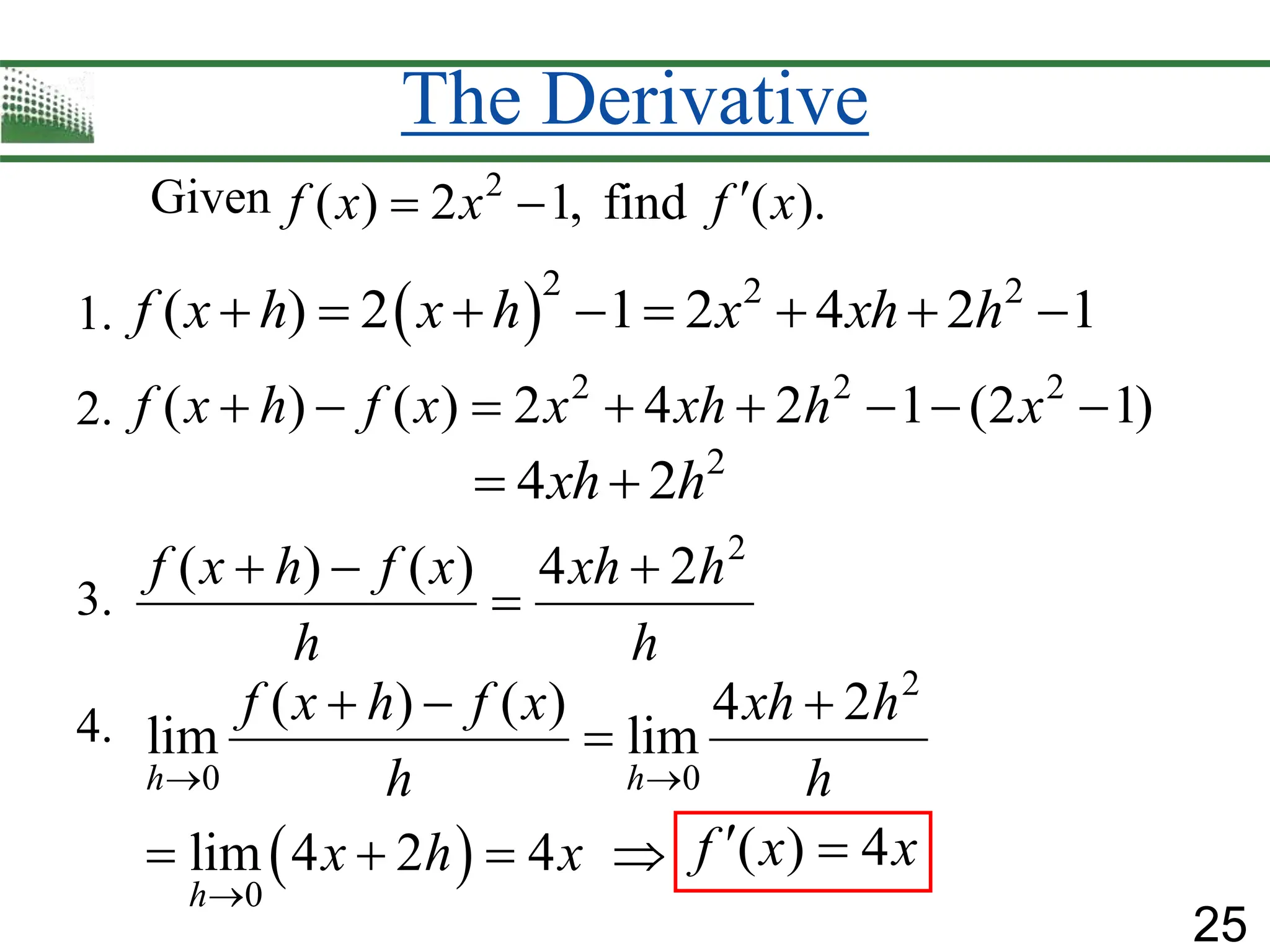
Given
2 2 2
( ) ( ) 2 4 2 1 (2 1)
f x h f x x xh h x
       
2
( ) ( ) 4 2
f x h f x xh h
h h
  

 2 2 2
( ) 2 1 2 4 2 1
f x h x h x xh h
       
1.
2.
3.
4.
2
( ) 2 1, find ( ).
f x x f x

 
2
4 2
xh h
 
( ) 4
f x x
 
26
Example
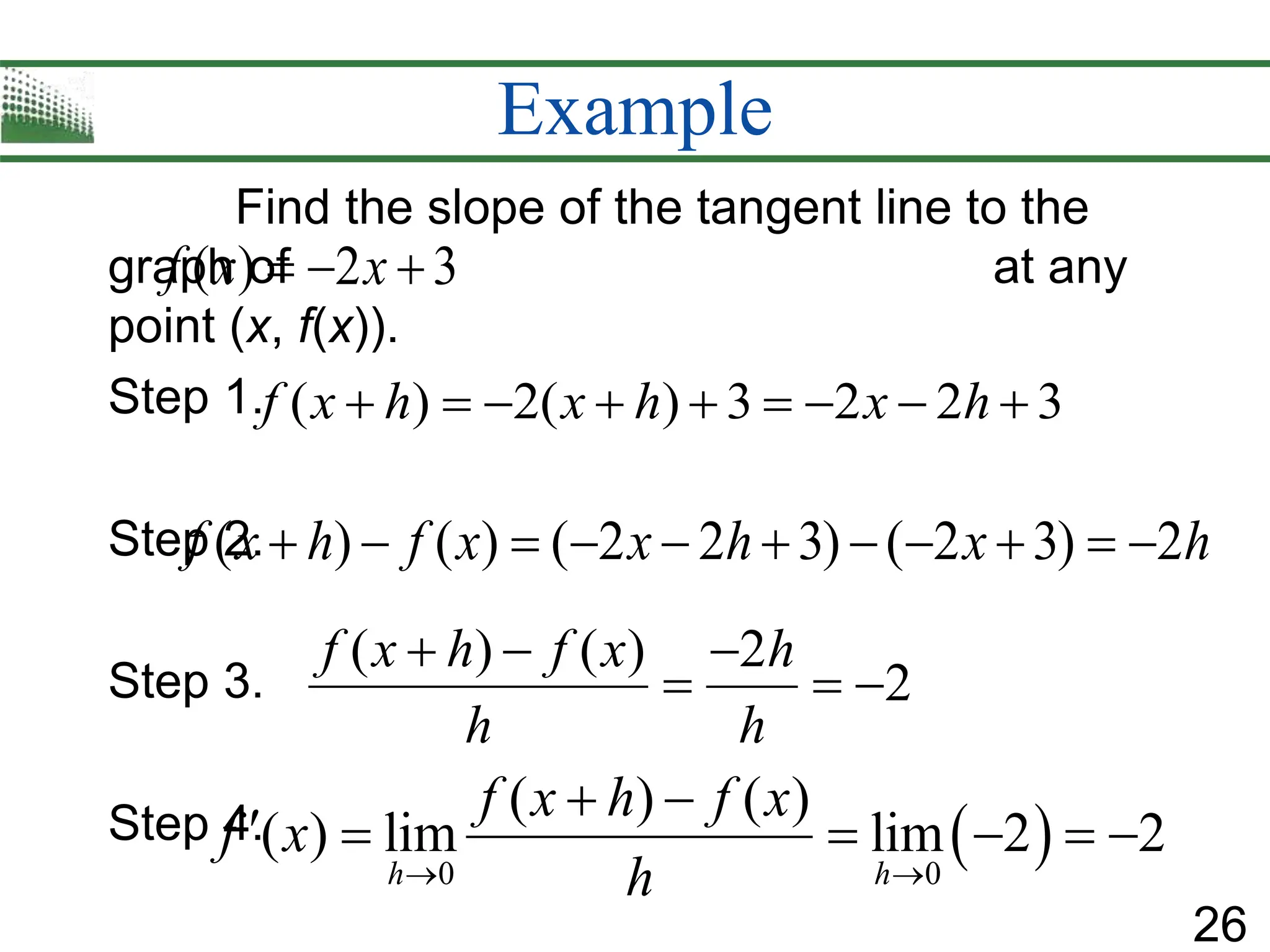
Find the slope of the tangent line to the
graph of at any
point (x, f(x)).
Step 1.
Step 2.
Step 3.
Step 4.
( ) 2( ) 3 2 2 3
f x h x h x h
        
( ) ( ) 2
2
f x h f x h
h h
  
  
( ) 2 3
f x x
  
( ) ( ) ( 2 2 3) ( 2 3) 2
f x h f x x h x h
          
 
0 0
( ) ( )
( ) lim lim 2 2
h h
f x h f x
f x
h
 
 
     
27
Differentiability and Continuity
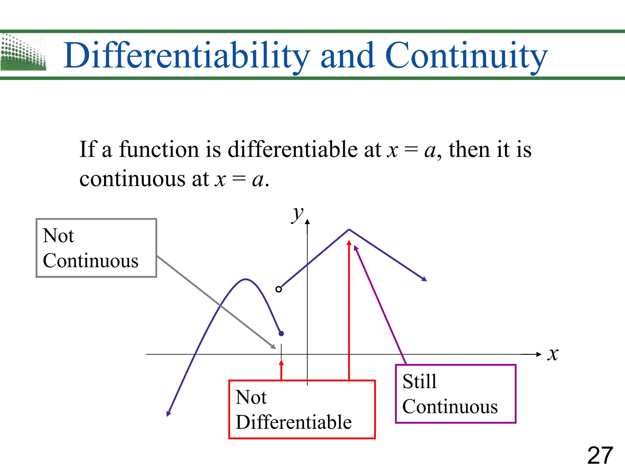
If a function is differentiable at x = a, then it is
continuous at x = a.
Not
Differentiable
Not
Continuous
Still
Continuous
x
y
28
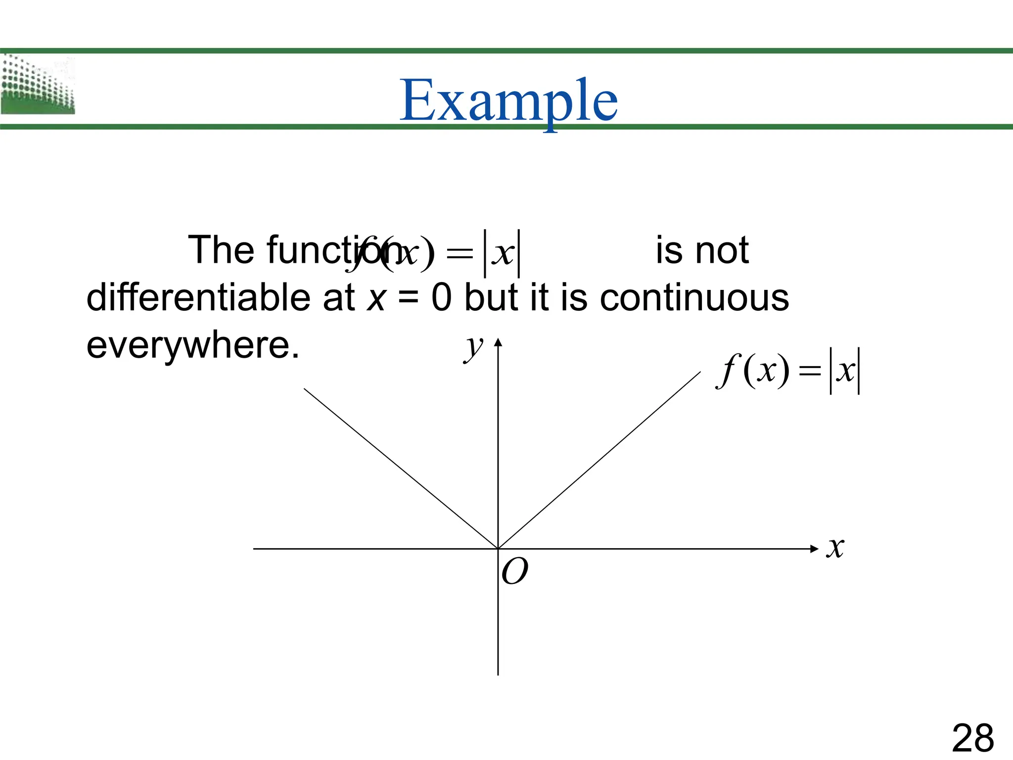
Example
The function is not
differentiable at x = 0 but it is continuous
everywhere.
( )
f x x

x
y
O
( )
f x x

29
Axiomas de Probabilidad
Dado un espacio muestral W , la probabilidad P de un
evento A es un número real no negativo P(A), que debe
satisfacer los tres axiomas siguientes:
• Límites
• Límites Laterales
• Continuidad
• La Derivada
30

LÍMITES Y DERIVADAS aplicados a ingenieria

  • 1.
  • 2.
    2 Límites y laDerivada • Límites • Límites Laterales • Continuidad • La Derivada
  • 3.
    3 Introducción al Cálculo Existendos áreas principales de interés: 1. Encontrar la recta tangente a una curva en un punto dado. ( ) y f x  Recta tangente   1 1 , x y 2. Encontrar el área de una región plana acotada por una curva. Área x x y y
  • 4.
    4 Velocidad Promedio Distancia recorrida Tiempotranscurrido  Instantánea Cuando el tiempo transcurrido se aproxima a cero Sobre cualquier intervalo de tiempo Si viajo 200 millas en 5 horas, mi velocidad promedio es 40 millas/hora. Cuando veo al oficial de policia, mi velocidad instantánea es 60 millas/hora. Distancia recorrida Tiempo transcurrido 
  • 5.
    5 Velocidad Ej. Given theposition function   2 10 s t t t   where t is in seconds and s(t) is measured in feet, find: a. The average velocity for t = 1 to t = 3. b. The instantaneous velocity at t = 1. ave (3) (1) 39 11 Velocity 14 ft/sec 3 1 2 s s       Average velocity t ( ) (1) 1 s t s t   1.1 12.1 1.001 12.001 1.01 12.01 Answer: 12 ft/sec  Notice how elapsed time approaches zero
  • 6.
    6 Límite de unaFuncción The limit of f (x), as x approaches a, equals L written: if we can make the value f (x) arbitrarily close to L by taking x to be sufficiently close to a. lim ( ) x a f x L   a L ( ) y f x  x y
  • 7.
    7 Computing Limits Ex. 2 3 if2 lim ( ) where ( ) 1 if 2 x x x f x f x x           6 -2 2 2 lim ( ) = lim 3 x x f x x    2 3 lim 3( 2) 6 x x        Note: f (-2) = 1 is not involved x y
  • 8.
    8 Properties of Limits      Suppose lim ( ) and lim ( ) Then, 1. lim ( ) , real number 2. lim ( ) lim ( ) , real number 3. lim ( ) ( ) 4. lim ( ) ( ) lim ( ) ( ) 5. lim ( ) lim x a x a r r x a x a x a x a x a x a x a f x L g x M f x L r a cf x c f x cL c a f x g x L M f x g x LM f x f x g x                    Provided that 0 ( ) x a L M g x M   
  • 9.
    9 Computing Limits Ex. Ex.   2 3 lim1 x x   2 3 3 lim lim1 x x x       2 3 3 2 lim lim1 3 1 10 x x x        1 2 1 lim 3 5 x x x        1 1 lim 2 1 lim 3 5 x x x x      1 1 1 1 2lim lim1 3lim lim5 x x x x x x        2 1 1 3 5 8    
  • 10.
    10 Indeterminate Form: 0 0 2 5 5 lim 25 x x x    Ex. Noticeform 0 0    5 5 lim 5 5 x x x x        5 1 1 lim 5 10 x x      Factor and cancel common factors
  • 11.
    11 Limits at Infinity Forall n > 0, 1 1 lim lim 0 n n x x x x     provided that is defined. 1 n x Ex. 2 2 3 5 1 lim 2 4 x x x x     2 2 5 1 3 lim 2 4 x x x x      3 0 0 3 0 4 4       Divide by 2 x 2 2 5 1 lim 3 lim lim 2 lim lim 4 x x x x x x x x                           
  • 12.
    12 One-Sided Limit ofa Function The right-hand limit of f (x), as x approaches a, equals L written: if we can make the value f (x) arbitrarily close to L by taking x to be sufficiently close to the right of a. lim ( ) x a f x L    a L ( ) y f x 
  • 13.
    13 One-Sided Limit ofa Function The left-hand limit of f (x), as x approaches a, equals M written: if we can make the value f (x) arbitrarily close to M by taking x to be sufficiently close to the left of a. lim ( ) x a f x M    a M ( ) y f x  x y
  • 14.
    14 One-Sided Limit ofa Function 2 if 3 ( ) 2 if 3 x x f x x x         Ex. Given 3 lim ( ) x f x   3 3 lim ( ) lim 2 6 x x f x x       2 3 3 lim ( ) lim 9 x x f x x       Find Find 3 lim ( ) x f x  
  • 15.
    15 Continuity of aFunction A function f is continuous at the point x = a if the following are true: ) ( ) is defined i f a ) lim ( ) exists x a ii f x  )lim ( ) ( ) x a iii f x f a   a f(a) y x
  • 16.
    16 Properties of ContinuousFunctions The constant function f (x) is continuous everywhere. Ex. f (x) = 10 is continuous everywhere. The identity function f (x) = x is continuous everywhere.
  • 17.
    17 Properties of ContinuousFunctions A polynomial function y = P(x) is continuous at everywhere. A rational function is continuous at all x values in its domain. ( ) ( ) ( ) p x R x q x  If f and g are continuous at x = a, then   , , and ( ) 0 are continuous at . f f g fg g a g x a   
  • 18.
    18 Intermediate Value Theorem Iff is a continuous function on a closed interval [a, b] and L is any number between f (a) and f (b), then there is at least one number c in [a, b] such that f(c) = L. ( ) y f x  a b f (a) f (b) L c f (c) = x y
  • 19.
    19 Intermediate Value Theorem  2 Given ( ) 3 2 5. Show that ( ) 0 has at least one solution on 1, 2 . f x x x f x     Ex. (1) 4 0 and (2) 3 0 f f      f (x) is continuous for all values of x and since f (1) < 0 and f (2) > 0, by the Intermediate Value Theorem, there exists a c on (1, 2) such that f (c) = 0.
  • 20.
    20 Existence of Zerosof a Continuous Function If f is a continuous function on a closed interval [a, b], and f(a) and f(b) have opposite signs, then there is at least one solution of the equation f(x) = 0 in the interval (a, b). f(b) f(a) a b x y
  • 21.
    21 Example (Existence of zerosof a continuous function) 1. Show that f(x) is a continuous function everywhere. The function is a polynomial function and is therefore continuous everywhere. 2. Show that f(x) = 0 has at least one solution on the interval (0, 2) Since (0) 5 and (2) 5 have opposite signs, there must be at least one number with 0 2 such that ( ) 0. f f x c c f c        2 Let ( ) 3 5. f x x x   
  • 22.
    22 Rates of Change Averagerate of change of f over the interval [x, x+h] ( ) ( ) f x h f x h    Instantaneous rate of change of f at x Slope of the Tangent Line Slope of Secant Line 0 ( ) ( ) lim h f x h f x h    
  • 23.
    23 The Derivative 0 ( )( ) ( ) lim h f x h f x f x h      The derivative of a function f with respect to x is the function , f  given by It is read “f prime of x.”
  • 24.
    24 The Derivative 0 ( )( ) ( ) lim h f x h f x f x h      Four-step process for finding : f  ( ) ( ) f x h f x   ( ) ( ) f x h f x h   ( ) f x h  1. Compute 2. Find 3. Find 4. Compute
  • 25.
    25 The Derivative   2 00 0 ( ) ( ) 4 2 lim lim lim 4 2 4 h h h f x h f x xh h h h x h x            Given 2 2 2 ( ) ( ) 2 4 2 1 (2 1) f x h f x x xh h x         2 ( ) ( ) 4 2 f x h f x xh h h h      2 2 2 ( ) 2 1 2 4 2 1 f x h x h x xh h         1. 2. 3. 4. 2 ( ) 2 1, find ( ). f x x f x    2 4 2 xh h   ( ) 4 f x x  
  • 26.
    26 Example Find the slopeof the tangent line to the graph of at any point (x, f(x)). Step 1. Step 2. Step 3. Step 4. ( ) 2( ) 3 2 2 3 f x h x h x h          ( ) ( ) 2 2 f x h f x h h h       ( ) 2 3 f x x    ( ) ( ) ( 2 2 3) ( 2 3) 2 f x h f x x h x h              0 0 ( ) ( ) ( ) lim lim 2 2 h h f x h f x f x h          
  • 27.
    27 Differentiability and Continuity Ifa function is differentiable at x = a, then it is continuous at x = a. Not Differentiable Not Continuous Still Continuous x y
  • 28.
    28 Example The function isnot differentiable at x = 0 but it is continuous everywhere. ( ) f x x  x y O ( ) f x x 
  • 29.
    29 Axiomas de Probabilidad Dadoun espacio muestral W , la probabilidad P de un evento A es un número real no negativo P(A), que debe satisfacer los tres axiomas siguientes: • Límites • Límites Laterales • Continuidad • La Derivada
  • 30.