1) The document discusses different variants of first order systems including: a) systems with non-unity steady state gain, and b) systems with time delay. 2) It then introduces second order systems, defined by a governing differential equation involving natural frequency, damping ratio, and input. 3) Based on the damping ratio value, second order systems can have complex conjugate poles (underdamped, ratio between 0-1), repeated real poles (critically damped, ratio equals 1), or distinct real poles (overdamped, ratio above 1). The implications of these cases will be explored next.

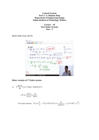
1. Control Systems
Prof. C. S. Shankar Ram
Department of Engineering Design
Indian Institute of Technology, Madras
Lecture – 18
First Order Systems
Part – 2
(Refer Slide Time: 00:18)
Other variants of 1st
Order system:
1) T
dy(t)
dt
+ y(t )=bu(t ),b∈ R,b≠1
→P(s)=
Y (s)
U (s)
=
b
Ts+1
Unit step response: U (s)=
1
s
,→Y (s)=P(s)U (s)=
b
s(Ts+1)
→ y (t)=b(1−e
−t
T
)

2. (Refer Slide Time: 00:30)
The steady state value of unit step response =
y (t )=lim
s→ 0
sY (s)=¿lim
s→0
s
b
s(Ts+1)
=b
lim
t→∞
¿
The dynamic characteristics remains the same; the settling time is still 4T, but now what will
happen you will see that if you substitute t = T, y(t) will be b times 0.632, that is why the
definition was 63.2 percent of the final value not just 0.632, if you look at the definition.
Similarly, if you calculate what is y at t = 4 t you will get 0.982 b. So, the output at our reach
98.2 percent of the final value which is b. So, that is what is called by steady state gain.
So, immediately you will see that this is a 2 parameter model; 2 parameter model or 2
parameter process, ok. So, this people call first order model with non unity steady state gain
right. So, that is the variant and a third variant which people can have which essentially
occurs in many practical processes you will see you will look at this variant even when you
come to the lab in many practical systems you may have a system like this.
2) T
dy(t)
dt
+ y(t )=bu(t−Td ),b∈ R,b≠1,Td>0,Td ∈R
So, Td is the time delay all right. So, we have encountered what was time delay before,
right. So, that is you give an input; output starts from 0 only after the interval of Td , right.
So, that is time delay.

3. Plant Transfer Function: P(s)=
Y (s)
U (s)
=
be
−Td s
Ts+1
=
b(2−Td s)
(Ts+1)(2+Td s)
(using Pade’s
approximation)
Now, how many parameters do we have? We have 3 parameters. So, this becomes a 3
parameter model ok. So, that is that is another variant, ok. So, this people will call as a first
order system with the non unity gain and time delay, ok. Some in chemical engineering
references and all you will see first order process plus time delay, ok. So, that is a term which
they will use ok. So, this is the model which is used and this is the transfer function which
comes over as a result ok. So, you see that you have 3 parameters.
So, once again the dynamic characteristics remain, the same the time constant definition is
the same. The steady state gain is once again b, only difference is and now we have added a
time delay factor, ok. So, that is that is the change that happens ok, is it clear?
(Refer Slide Time: 09:51)
So, now, we go to second order systems. So, once again to recap the big picture as to why we
are studying first order and second order systems the reason is that by and large when you
want to talk about performance right we talk about the fact that we have the dominant
dynamics or dominant poles to be either one or two other is like what is close to the
imaginary axis, right. That is why when you want to specify performance we look at either
first order or second order systems you know like that is the motivation behind looking at

4. first order and second order systems for deriving performance parameters, ok. So, that is the
big picture once again.
Second Order Systems:
So, a typically second order systems are motivated from vibration problems. Due to that
reason their governing equation is written in a certain structure ok, we will see how it is
written, ok. So, the governing equation of second order systems is typically taken as the
following,
d
2
y(t)
d t
2
+2ζ ωn
dy(t)
dt
+ωn
2
y(t )=ωn
2
u(t )
So, immediately you can see that n = 2, right. So, m for this particular case happens to be 0,
you can also have = 1, you can also have a derivative of u on the right hand side. can happen
as I told you we we would take it of to be of this particular structure and we will see what
happens when we have m to be 1, that is we have a term on the right hand side what really
happens to the systems response, that is something which we look at as we go along, ok.
So, we can see that immediately of course, before we calculate the poles you know like the
value ζ is what is called as the damping ratio ok, ωn is what is called as the natural
frequency of the system, ok. We would revisit these parameters and then I would ask you to
define these parameters like we are going to look at the physics behind these choices, right.
So, behind this choice of model, right, we will we will look at them. But, then like for
tomorrows or let us say for the next class you know I should say you know like please figure
out what is the definition of natural frequency and come, ok. So, a clear crisp definition of
what you mean by natural frequency, we discuss this as we go along.
And it so happens that we will we will figure out later that for stability of the system please
remember we can only talk about performance only if you have a stable system to begin with
right. It so happens that for stability of this class of systems the sufficient condition is ζ >
0, ωn>0 , ok. So, that is the sufficient condition of course, in general we will see that you
know like the system will be stable if ζ and ωn are real numbers of the same sign, ok.
Now, taking Laplace transform on both sides,
s
2
Y (s)−sy (0)−´y(0)+2ζ ωn(sY (s)− y(0))+ωn
2
Y (s)=ωn
2
U (s)

5. Apply zero initial conditions,
s
[¿¿2+2ζ ωn s+ωn
2
]Y (s)=ωn
2
U (s)
¿
→P(s)=
Y (s)
U (s)
=
ωn
2
s
2
+2ζ ωn s+ωn
2
So, what are the poles of this transfer function? How do you get the poles? We solve the
denominator polynomial equals 0
Poles: s=−ζ ωn±ωn√ζ
2
−1 .
Now, of course, it is a second order system value of n is 2; obviously, you get two poles,
right. Now, what can you say about these nature of these poles?
Immediately we can observe that the nature of the poles is depend on the value of zeta, right.
If zeta is between 0 and 1, what can I say about the poles?
If 0<ζ <1 the poles are complex conjugates
If ζ =1 Repeated poles at −ωn
If ζ >1 Distinct real poles.
So, those are three cases that we would look at depending on the value of zeta the location of
the poles changes and consequently the system behavior changes a lot, ok.
So, that is something which we are going to do in the next class. So, we look at what are
called under damped critically damped and over damped systems, depending on whether the
value of ζ is less than 1, exactly equal to 1 or greater than 1, respectively, ok. So, we look
at what is the physical what to say implication of those three cases and then how do we do the
analysis, ok. So, that is something which we will do in the next class, but before that you
know like please figure out the definitions of a natural frequency and damping ratio, and
come.