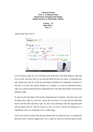
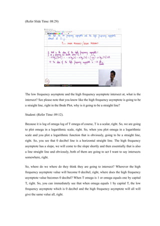
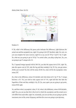
Control Systems
Prof. C. S. Shankar Ram
Department of Engineering Design
Indian Institute of Technology, Madras
Lecture – 51
Bode Plot 2
Part - 1
(Refer Slide Time: 00:17)
Let us continue, right. So, we are looking at the Bode Plot or the bode diagram, right and
if you recall, you know like we saw that the Bode Plot has two plots; a magnitude plot
and a phase plot and one of the big advantage of plotting the magnitude in decibels is
that like if we have the transfer function as a product or a ratios of individual blocks,
right, one could essentially plot the magnitude plot of the individual blocks and then just
add them, right.
So, that was the advantage of having the magnitude plot in decibels. And same story with
the phase plot, right. So, you have a phase plot you know if we just plot the individual
factors and then like add them, right. So, that is the advantage with the magnitude plot
and the phase book ok. And the reason we why we want to choose the frequency in a
logarithmic scale is to essentially cover a wider range.
And if you recall, you know like the basic factors that we looked at were 3 a constant the
derivative term s and the integral term 1 by s, right. So, these are the three factors which
you have looked at till now, right. So, today, let us proceed and look at the next factor ok.
So, see what numbering did I use there. So, just to ensure that I am consistent ok, I used
3 ok.
(Refer Slide Time: 01:43)
So, let us say as the fourth factor, let us say we choose a G of s to be 1 by T s plus 1 ok.
So, first order term, right. So, of course, we have 1 by T s plus 1, you know like and let
us basically consider of course, T to be greater than 0, we will see what happens when T
becomes negative ok, later on, right. So, to begin with we will consider that T is are a
positive real number ok.
So, let us say we have 1 by T s plus 1 as our factor. So, what will happen to G of j
omega? Please recall that we are dealing with the sinusoidal transfer function, right. So,
you substitute s equals j omega. So, this is going to become 1 divided by 1 plus j times T
omega. So, this can be written as rewritten as 1 minus j T omega divided by 1 plus T
square omega square, right when I multiply by the conjugate factor ok. So, this is what is
going to happen.
So, consequently, what will happen to the magnitude of G of j omega? So, from this
factor, we know that it is going to be the ratio of the individual magnitudes. So, I can
write rewrite this as 1 divided by square root of 1 plus T square omega square, right. So,
that is pretty straightforward and the phase of G of j omega is going to be minus tan
inverse of T omega, right. So, that is going to be the magnitude and phase of this
particular factor ok.
So, one can observe that you know like as we go to more slightly complex terms, you
know like the expressions become a little bit more involved, right. So, but then we are
going to do some simplifications, right. So, let us look at the magnitude first and then we
will go to the phase ok. So, this is what we have as a magnitude and phase of this first
order term, right.
So, now let us look at the magnitude term ok. So, we are going to look at this magnitude
term ok. So, at low frequencies, where when omega is very very small when compared to
1 by T, we will see why I am choosing 1 by capital T as a as a particular value, right in
this expression ok. So, when omega is very much lower than 1 by capital T, what do you
think is going to happen to this magnitude?
So, we can immediately see that the magnitude of G of j omega is going to tend to 1,
right why? Because, let us say when omega is less than 1 by T you can immediately, see
that T omega is very very small then compared to 1. Then what can you say about 1 plus
T square omega square T, if T omega is very small you know like 1 plus T, T squared
omega squared is going to be even smaller. Let us say T omega is 0.01. What is going to
happen to T square omega squared? It is going to become 10 power minus 4, right.
So, 1 plus 10 power minus 4, I can approximate it as 1 itself, right. So, the magnitude is
going to tend to 1 or equivalently 0 decibels, right in decimal units, it is going to tend to
0 decibels. Do you agree? See because, how do I convert to decimal units. I take the
logarithm to the base 10 and multiply by 20; right logarithm of one is going to be 0,
right. So, that is why I get 0 decibels ok.
So, we would see that the magnitude of the, this particular factor is going to tend to a line
which corresponds to the 0 decibel line in the magnitude plot as frequencies become
smaller and smaller when compared to 1 by capital T ok. So, for this reason, this
particular value or locus is going to be denoted as the low frequency asymptote. So, this
is what is called as a low frequency asymptote. So, why is it called, because it tends to
this value, right as omega is very very small at low frequencies, right?
So, that is why the 0 decibel line in the magnitude plot is called as the low frequency
asymptote. Now, at high frequencies what do I mean by high frequencies, you know like
when omega is much much greater than 1 by T; of course, when omega is much greater
than 1 by T what is going to happen to T omega, you can really see that T omega is going
to be much much greater than 1. Then let us say T omega is let us say 10 power 2 let us
say 100, right T squared omega squared is going to become 10 power 4.
So, what can you say about 1 plus T squared omega squared. I can say that it is going to
be 1 plus 10 power 4. That is almost 10 power 4, right. So, I can say that I am going to
approximate 1 plus T squared omega squared T squared omega squared itself, right. So,
what is going to happen to this magnitude? So, immediately we can observe that the
magnitude of G of j omega tends to 1 by T omega, I hope it is clear how we got this,
right
So, or in decibel measures, it is going to be minus 20 log to the base 10 T omega
decibels, right because you take logarithm to the base 10, you will get minus log 10 T
omega and multiplied by 20 ok. That is how you get this measure, right. So, this is the
value to which the magnitude will tend to at high frequencies, right. So, that is why it is
called as a high frequency asymptote ok.
So, I hope it is clear what are low frequency and high frequency asymptotes, right. So,
essentially we are looking at what happens to this magnitude and frequency is lower than
1 by capital T and higher than 1 by capital T. And why did I choose capital T and 1 by
capital T here? You know like, please remember for a first order factor 1 by T s plus 1,
right capital T greater than 0, you know like if you recall the physical significance of
capital T that was a time constant, right of a first order system, right.
So, if you recall a plant transfer function of the form 1 by capital T s plus 1, right yeah.
So, why did I consider 1 by capital T, you know like we can note that.
(Refer Slide Time: 08:29)
The low frequency asymptote and the high frequency asymptote intersect at, what is the
intersect? See please note that you know like the high frequency asymptote is going to be
a straight line, right in the Bode Plot, why is it going to be a straight line?
Student: (Refer Time: 09:12).
Because it is log of omega log of T omega of course, T is a scalar, right. So, we are going
to plot omega in a logarithmic scale, right. So, when you plot omega in a logarithmic
scale and you plot a logarithmic function that is obviously, going to be a straight line,
right. So, you see that 0 decibel line is a horizontal straight line. The high frequency
asymptote has a slope, we will come to the slope shortly and then essentially that is also
a line straight line and obviously, both of them are going to act I want to say intersects
somewhere, right.
So, where do we where do they think they are going to intersect? Wherever the high
frequency asymptote value will become 0 decibel, right, where does the high frequency
asymptote value becomes 0 decibel? When T omega is 1 or omega equals one by capital
T, right. So, you can immediately see that when omega equals 1 by capital T, the low
frequency asymptote which is 0 decibel and the high frequency asymptote will all will
give the same value all, right.
So, essentially in principle, they are intersecting each other, right. So, this is what is
called as a Corner Frequency or some people will call it as the Break Frequency. See one
thing which you should be careful about when you do practical problems is that like all
this frequency omega should be in radians per second ok. So, that is a very very common
thing where people can make a mistake because typically, we talk about frequency in
Hertz, right. But, when you talk about omega, it is going to be 2 pi f, right. So, you need
to convert that frequency given and Hertz into radians per second please remember that
when you do practical problems ok. So, this is essentially what is called as a corner
frequency or a break frequency, is it clear ok.
Now, you know let us let us plot them, right. So, essentially, but before we plot let us ask
ourselves the question, right. So, the question that we are going to ask ourselves is that
what is the slope of the high frequency asymptote? Ok, let us ask ourselves a question
what, what should be the slope of the high frequency asymptote, right. So, the high
frequency asymptote is going to be minus 20 log to the base 10 T omega, right.
So, what is the slope? So, of course, a common way to find the slope is it like, let us say
as we discuss you know it is going to be expressed in Decibels per Decade or decibels
per octave. Typically, we express in decibels per decade. So, what you do you choose a
particular omega and go to 10 times omega and then find out what is the difference,
right. So, that is say whatever is the difference is the value of the slope in Decibels per
Decade, right.
So, let us look at that. So, if I go from omega to 10 times omega, let us say from T
omega to T times 10 omega. So, what am I going to gain? What will happen to this?
Here I can rewrite this as minus 20 log to the base 10 minus 20 log to the base 10 or T
omega and what is the first term, it is going to be minus 20 and minus 20 log to the base
10, right.
So, what did I do, you know like this to answer this you know like to be more formal at a
frequency one decade above omega, this is going to be this. So, what do you think is a
slope? The slope of the high frequency asymptote is going to be minus 20 decibels per
decade, right why because you can see this, right. So, you are going to have a difference
of minus 20 from omega to 10 times omega, right.
So, consequently the slope of the high frequency asymptote is minus 20 decibels per
decade ok. That is what we have fine ok. So, that is what we have as the slope of the high
frequency asymptote, right. So, of course, what is the slope of the low frequency
asymptote?
Student: 0.
0, right it is just a flat line, right on the in the in the plot, right the magnitude plot. So, let
us plot these two things ok.
(Refer Slide Time: 14:08)
So, let us plot them. So, let us draw the magnitude plot, will then come to the phase plot,
right. So, first let me plot the magnitude plot. So, let us say this is omega; this is
magnitude of G of j omega in decibels, right.
Let us say this is let us say this I call a 0 ok, let us say, this I call as minus 20, right, so,
20 minus 40 and so on ok. So, similarly let us say I, I take a frequency 1 by capital T, I
take a frequency 10 by capital T and I take a frequency point 1 by capital T you know
like I am just looking at a region one decade are born below the corner frequency, right.
So, I can do this I am just plotting 1 by capital T.
So, let us let us plot the low frequency, high frequency and the actual curves, right. So,
see the low frequency asymptote which I am indicating in pink. So, is the 0 decibel line
right. So, it does not matter what the frequency is; of course, it makes sense only at the
low frequency, but then I am just drawing it ok, so, just to make the things clear, right.
So, the 0 decibel line or the pink line is the low frequency asymptote. Of course, it makes
sense only at low frequencies, right. Just for the sake of clarity, I just extended it, right.
So, what about the high frequency asymptote? The high frequency asymptote once again
makes sense only after a 1 by capital T. So, how do I draw it? At 1 by capital T, the value
of 0 decibels, right; 10 by capital T, it is going to be minus 20, right. So, I I plot minus
twenty. So, essentially I draw a straight line which passes through these two watts ok.
So, this is the high frequency asymptote ok; the one and golden color, right. So, this is
the high frequency asymptote ok. So, of course, the slope of this line is going to be
minus 20 decibels per decade ok. That is what we are going to have fine ok. Now, they
are both of them intersected 1 by capital T ok. So, for drawing Bode Plots by hand, as far
as problems in your homework, exams and are concerned, you need to only plot the
symptoms and use the asymptotes curve as your approximation of the Bode Plot for that
particular factor.
So, what I am going to draw is the first approximation ok. So, what is the
approximation? I am just going to draw by a solid what we say curve. So, let us say, so,
the approximation of the factor 1 by T s plus 1 is going to be this ok. So, it is going to
remain 0 decibels still 1 by capital T and after 1 by capital T it is going to essentially
reduce at the rate of minus 20 decibels per decade.
So, what I have drawn in the maroon solid line is the asymptotic approximation of G of 1
by T s plus 1. The magnitude of 1 by T s plus 1 to be very very, 1 by T j omega plus 1
that that is what I have done ok, but that is enough for drawing by hand as far as the
exams and homeworks are concerned ok, but what about the real curve, right. So, how
does it look, right because see this is like basically a non-smooth curve, right because
why although, it is continuous, at omega equals 1 by T, you suddenly have the slope
changing alright.
But the real function is a smooth function, right. So, it is basically what is the actual
magnitude? You can see that that is going to be 1 by 1 plus T square omega square, right.
So, let us let us figure that one out, right. So, how do I do that? So, far in that exercise
you know like, please calculate and tell me what values you see. So, let us say at omega I
am going to construct a table ah. So, the actual magnitude and decibels and the
asymptotes value in decibels also ok. So, what I want you to do is that like please
calculate at 1 by T, right and 2 by T 0.5 by T ok.
So, please calculate that these three values and let me know ok. So, can you do that
please?
Student: (Refer Time: 09:27).
Because it makes sense only after 1 by capital T, right. So, yeah if you want graphically
you know like a representation, say physically it does not make sense, right. See these
are symptotes that is the step, but then you should not treat it as an asymptote any farther
it is just a line, right. So, please note that the high frequency asymptote makes sense only
when omega tends to infinity, right.
Similarly, the pink low frequency asymptote makes sense only when omega tends to 0.
Here you just look at some like two lines which are intersecting ok. So, that I want to
provide you with a graphical visualization, right. So, yeah let us let us look at, can you
tell me what are the values you get?
Student: Sure.
Yeah.
Student: Yeah symptotes approximation (Refer Time: 20:18).
That is what we have, please calculate, good point. That is exactly the purpose behind
this exercise ok, yeah. Let us see how huge is deviations, right ok. So, what do you think
will happen to the value of magnitude of G of j omega, the actual one, right. So, in
decibels, see what is the magnitude of G of j omega I think I should scroll up a little bit I
should scroll down a little bit, right. So, yeah I think. So, that it is visible.
Let me erase this. Please note that the actual magnitude of G of j omega in decibels is
going to be minus 20 log to the base 10 square root of 1 plus T squared omega square,
right, if this asset is, right no approximation. So, now, substitute omega equals 1 by
capital T there, what do you get? You get log of square root of 2, right. What is that?
So, that that you can say as minus 10 log of 2 what is log of 2.
Student: Point.
0.3010, right to the base 10, so, I can say that this is going to be minus 3.01 decibel and
what is the asymptotes value.
Student: 0.
0, right. So, consequently, what is the change the error the magnitude of the error is
going to be sorry minus 3.101 decibel ok, difference oops sorry. So, let me write it
clearly. So, the difference is going to be minus 3 decibels, right do you agree?
So obviously, between the asymptotic approach and the actual curve, you are going to
have minus 3 decibels. So, the idea is that like if you want to be very particular, you can
apply this correction. See please remember see, why am I doing all these things?
Suppose let us imagine that we do not have a computer, right we do not have access to a
computer, you need to draw by hand and take do control design and take some calls,
right.
So, you can follow this approach, right. But, but you should also have an intuitive idea,
right say someone let us say tomorrow, I give you a bode diagram and then I ask you to
figure out the transfer function, right. So, if you know these concepts, you would be able
to a hypothesize what should be the potential transfer function, right. So, that is also
another object of why we are doing these exams, right.
So, now calculate a 2 by T. What is 2 by T when compared to 1 by T? One octave, right
beyond the corner frequency, right; so, can you calculate what is going to be magnitude
of G of j omega in decibels? So, you substitute and then you get square root of 5, right
ah. So, what is minus 10 log of 5. Can someone calculate and tell me?
Student: Log of 5.6.
Do you have a calculator? No. So, log of 5 is 0.69 yeah, right. So, then I multiply by 10 I
am going to get minus 6 point let us say tan 9, right. So, it is going to be close to minus
7, right so, but anyway I will write this value it is going to be minus 6 point, minus 6
point let us say 9, 9, let me round it off, right decibels ok.
So, what is asymptotes value? Where will you substitute for the asymptote value? You
will substitute in the high frequency asymptote why because now the omega is greater
than the corner frequency. So, I can say absent or value 0 decibels. I have to use a high
frequency asymptote. What a high frequency asymptote? It is minus 20 log T omega.
So, you substitute omega equals 2 by capital T in that whatever you going to get you are
going to get minus 20 log 2, right because please recall, the high frequency asymptote is
going to be minus 20 log T omega in decibels, right for the high frequency asymptote.
So, when you substitute omega equals 2 by capital T, you get minus 20 log 2, right.
So, what is minus 20 log 2, let us quickly calculate that, right. So, although it is going to
be pretty straightforward, but let us do that, right. So, so I am going to get 0.3010, right
multiply by 20, you get almost around 6 all, right. So, we are going to get our on like
6.02 decibels, right. So, this is going to be minus 6.02.
So, what do you think is a difference between the two? It is going to be 0.97, right. So,
now, can you calculate that 0.5 by T? Can you calculate it what happens to the actual
value at 0.5 by T. So, if you have to plug in that equation. So, T squared omega squared
is going to be 0.25, right. So, you take the square root of 1.25 and then multiply it by oh
no wait a minute.
So, essentially we have 1.25 square root then, you take the logarithm, right and then
multiply it by 20 that is what I am doing. So, I get 0. 97, right, minus 0.97 ok; so, what
will be the asymptotic value at 0.5 by capital T?
(Refer Slide Time: 26:15)
Student: 0.
0. So, what is the difference the green color indicates the difference, right between the
actual one and the asymptote one, right. It is going to be 0.97 decibels, right. So, now, we
you can complete the same exercise, right let us say you do 10 by T and 0.1 by T, right.
So, what are you going to get at 10 by T as actual value, you plug a plug here. So, you
are going to get T omega to be 10.
So, T squared omega squared will be 100. So, you take the square root of 101, right. So,
take the square root of 101, take the log and then multiply it by 20. So, you get minus
20.04, am I correct? So, this will be minus 20.04. So, what will be the asymptotes value
minus 20?
So, what is the difference, minus 0.4 decibels and what about at 0.1 by T? So, T omega
becomes a 0.1. So, you need to take square root of 1.01, right and then like take the
logarithm of that and then multiply it by 20. So, once again you are going to get point,
minus 0.04, right.
So, and then what is asymptotic value, 0. So, what is the difference, minus 0.04 decibels,
right? So, you can see that this is the level to which the asymptotes and the actual curve
will differ from each other, right. So, essentially, you can see that you are going to get the
maximum error at the corner frequency and then the errors are going to just decrease.
So, if you plot the error, this is omega. So, this is the error in decibels ok. So, what is
going to happen is then. So, if you have 1 by capital T, 10 by capital T and minus sorry.
So, not minus 0.1 by capital T, what is going to happen is that. So, let us say this is minus
3.01, right. So, you are going to have the maximum error here beyond that, you know
like you are going to have on either side a decreasing error profile, right which will
asymptotically tend to 0, right. That is what you are going to have as far as the difference
is concerned, right.
So, yes the drawing the asymptotes is only an approximation, but a reasonable
approximation, right. So, you are going to get any maximum error of 3 decibels, right in
magnitude, but that is you know like to you one kind if we are very particular, let us say
imagine a case where people did not have any computers, right let us say a century ago
correct and you wanted to create the bode diagram, right.
Let us say you take a piece of paper and you can apply these corrections and then draw a
smooth curve, right. So, that is that still you know like that is the best we could do, right.
So, that essentially takes care of the magnitude plot, right, is it clear any questions?

Lec51

  • 1.
    Control Systems Prof. C.S. Shankar Ram Department of Engineering Design Indian Institute of Technology, Madras Lecture – 51 Bode Plot 2 Part - 1 (Refer Slide Time: 00:17) Let us continue, right. So, we are looking at the Bode Plot or the bode diagram, right and if you recall, you know like we saw that the Bode Plot has two plots; a magnitude plot and a phase plot and one of the big advantage of plotting the magnitude in decibels is that like if we have the transfer function as a product or a ratios of individual blocks, right, one could essentially plot the magnitude plot of the individual blocks and then just add them, right. So, that was the advantage of having the magnitude plot in decibels. And same story with the phase plot, right. So, you have a phase plot you know if we just plot the individual factors and then like add them, right. So, that is the advantage with the magnitude plot and the phase book ok. And the reason we why we want to choose the frequency in a logarithmic scale is to essentially cover a wider range. And if you recall, you know like the basic factors that we looked at were 3 a constant the derivative term s and the integral term 1 by s, right. So, these are the three factors which
  • 2.
    you have lookedat till now, right. So, today, let us proceed and look at the next factor ok. So, see what numbering did I use there. So, just to ensure that I am consistent ok, I used 3 ok. (Refer Slide Time: 01:43) So, let us say as the fourth factor, let us say we choose a G of s to be 1 by T s plus 1 ok. So, first order term, right. So, of course, we have 1 by T s plus 1, you know like and let us basically consider of course, T to be greater than 0, we will see what happens when T becomes negative ok, later on, right. So, to begin with we will consider that T is are a positive real number ok. So, let us say we have 1 by T s plus 1 as our factor. So, what will happen to G of j omega? Please recall that we are dealing with the sinusoidal transfer function, right. So, you substitute s equals j omega. So, this is going to become 1 divided by 1 plus j times T omega. So, this can be written as rewritten as 1 minus j T omega divided by 1 plus T square omega square, right when I multiply by the conjugate factor ok. So, this is what is going to happen. So, consequently, what will happen to the magnitude of G of j omega? So, from this factor, we know that it is going to be the ratio of the individual magnitudes. So, I can write rewrite this as 1 divided by square root of 1 plus T square omega square, right. So, that is pretty straightforward and the phase of G of j omega is going to be minus tan
  • 3.
    inverse of Tomega, right. So, that is going to be the magnitude and phase of this particular factor ok. So, one can observe that you know like as we go to more slightly complex terms, you know like the expressions become a little bit more involved, right. So, but then we are going to do some simplifications, right. So, let us look at the magnitude first and then we will go to the phase ok. So, this is what we have as a magnitude and phase of this first order term, right. So, now let us look at the magnitude term ok. So, we are going to look at this magnitude term ok. So, at low frequencies, where when omega is very very small when compared to 1 by T, we will see why I am choosing 1 by capital T as a as a particular value, right in this expression ok. So, when omega is very much lower than 1 by capital T, what do you think is going to happen to this magnitude? So, we can immediately see that the magnitude of G of j omega is going to tend to 1, right why? Because, let us say when omega is less than 1 by T you can immediately, see that T omega is very very small then compared to 1. Then what can you say about 1 plus T square omega square T, if T omega is very small you know like 1 plus T, T squared omega squared is going to be even smaller. Let us say T omega is 0.01. What is going to happen to T square omega squared? It is going to become 10 power minus 4, right. So, 1 plus 10 power minus 4, I can approximate it as 1 itself, right. So, the magnitude is going to tend to 1 or equivalently 0 decibels, right in decimal units, it is going to tend to 0 decibels. Do you agree? See because, how do I convert to decimal units. I take the logarithm to the base 10 and multiply by 20; right logarithm of one is going to be 0, right. So, that is why I get 0 decibels ok. So, we would see that the magnitude of the, this particular factor is going to tend to a line which corresponds to the 0 decibel line in the magnitude plot as frequencies become smaller and smaller when compared to 1 by capital T ok. So, for this reason, this particular value or locus is going to be denoted as the low frequency asymptote. So, this is what is called as a low frequency asymptote. So, why is it called, because it tends to this value, right as omega is very very small at low frequencies, right?
  • 4.
    So, that iswhy the 0 decibel line in the magnitude plot is called as the low frequency asymptote. Now, at high frequencies what do I mean by high frequencies, you know like when omega is much much greater than 1 by T; of course, when omega is much greater than 1 by T what is going to happen to T omega, you can really see that T omega is going to be much much greater than 1. Then let us say T omega is let us say 10 power 2 let us say 100, right T squared omega squared is going to become 10 power 4. So, what can you say about 1 plus T squared omega squared. I can say that it is going to be 1 plus 10 power 4. That is almost 10 power 4, right. So, I can say that I am going to approximate 1 plus T squared omega squared T squared omega squared itself, right. So, what is going to happen to this magnitude? So, immediately we can observe that the magnitude of G of j omega tends to 1 by T omega, I hope it is clear how we got this, right So, or in decibel measures, it is going to be minus 20 log to the base 10 T omega decibels, right because you take logarithm to the base 10, you will get minus log 10 T omega and multiplied by 20 ok. That is how you get this measure, right. So, this is the value to which the magnitude will tend to at high frequencies, right. So, that is why it is called as a high frequency asymptote ok. So, I hope it is clear what are low frequency and high frequency asymptotes, right. So, essentially we are looking at what happens to this magnitude and frequency is lower than 1 by capital T and higher than 1 by capital T. And why did I choose capital T and 1 by capital T here? You know like, please remember for a first order factor 1 by T s plus 1, right capital T greater than 0, you know like if you recall the physical significance of capital T that was a time constant, right of a first order system, right. So, if you recall a plant transfer function of the form 1 by capital T s plus 1, right yeah. So, why did I consider 1 by capital T, you know like we can note that.
  • 5.
    (Refer Slide Time:08:29) The low frequency asymptote and the high frequency asymptote intersect at, what is the intersect? See please note that you know like the high frequency asymptote is going to be a straight line, right in the Bode Plot, why is it going to be a straight line? Student: (Refer Time: 09:12). Because it is log of omega log of T omega of course, T is a scalar, right. So, we are going to plot omega in a logarithmic scale, right. So, when you plot omega in a logarithmic scale and you plot a logarithmic function that is obviously, going to be a straight line, right. So, you see that 0 decibel line is a horizontal straight line. The high frequency asymptote has a slope, we will come to the slope shortly and then essentially that is also a line straight line and obviously, both of them are going to act I want to say intersects somewhere, right. So, where do we where do they think they are going to intersect? Wherever the high frequency asymptote value will become 0 decibel, right, where does the high frequency asymptote value becomes 0 decibel? When T omega is 1 or omega equals one by capital T, right. So, you can immediately see that when omega equals 1 by capital T, the low frequency asymptote which is 0 decibel and the high frequency asymptote will all will give the same value all, right.
  • 6.
    So, essentially inprinciple, they are intersecting each other, right. So, this is what is called as a Corner Frequency or some people will call it as the Break Frequency. See one thing which you should be careful about when you do practical problems is that like all this frequency omega should be in radians per second ok. So, that is a very very common thing where people can make a mistake because typically, we talk about frequency in Hertz, right. But, when you talk about omega, it is going to be 2 pi f, right. So, you need to convert that frequency given and Hertz into radians per second please remember that when you do practical problems ok. So, this is essentially what is called as a corner frequency or a break frequency, is it clear ok. Now, you know let us let us plot them, right. So, essentially, but before we plot let us ask ourselves the question, right. So, the question that we are going to ask ourselves is that what is the slope of the high frequency asymptote? Ok, let us ask ourselves a question what, what should be the slope of the high frequency asymptote, right. So, the high frequency asymptote is going to be minus 20 log to the base 10 T omega, right. So, what is the slope? So, of course, a common way to find the slope is it like, let us say as we discuss you know it is going to be expressed in Decibels per Decade or decibels per octave. Typically, we express in decibels per decade. So, what you do you choose a particular omega and go to 10 times omega and then find out what is the difference, right. So, that is say whatever is the difference is the value of the slope in Decibels per Decade, right. So, let us look at that. So, if I go from omega to 10 times omega, let us say from T omega to T times 10 omega. So, what am I going to gain? What will happen to this? Here I can rewrite this as minus 20 log to the base 10 minus 20 log to the base 10 or T omega and what is the first term, it is going to be minus 20 and minus 20 log to the base 10, right. So, what did I do, you know like this to answer this you know like to be more formal at a frequency one decade above omega, this is going to be this. So, what do you think is a slope? The slope of the high frequency asymptote is going to be minus 20 decibels per decade, right why because you can see this, right. So, you are going to have a difference of minus 20 from omega to 10 times omega, right.
  • 7.
    So, consequently theslope of the high frequency asymptote is minus 20 decibels per decade ok. That is what we have fine ok. So, that is what we have as the slope of the high frequency asymptote, right. So, of course, what is the slope of the low frequency asymptote? Student: 0. 0, right it is just a flat line, right on the in the in the plot, right the magnitude plot. So, let us plot these two things ok. (Refer Slide Time: 14:08) So, let us plot them. So, let us draw the magnitude plot, will then come to the phase plot, right. So, first let me plot the magnitude plot. So, let us say this is omega; this is magnitude of G of j omega in decibels, right. Let us say this is let us say this I call a 0 ok, let us say, this I call as minus 20, right, so, 20 minus 40 and so on ok. So, similarly let us say I, I take a frequency 1 by capital T, I take a frequency 10 by capital T and I take a frequency point 1 by capital T you know like I am just looking at a region one decade are born below the corner frequency, right. So, I can do this I am just plotting 1 by capital T. So, let us let us plot the low frequency, high frequency and the actual curves, right. So, see the low frequency asymptote which I am indicating in pink. So, is the 0 decibel line
  • 8.
    right. So, itdoes not matter what the frequency is; of course, it makes sense only at the low frequency, but then I am just drawing it ok, so, just to make the things clear, right. So, the 0 decibel line or the pink line is the low frequency asymptote. Of course, it makes sense only at low frequencies, right. Just for the sake of clarity, I just extended it, right. So, what about the high frequency asymptote? The high frequency asymptote once again makes sense only after a 1 by capital T. So, how do I draw it? At 1 by capital T, the value of 0 decibels, right; 10 by capital T, it is going to be minus 20, right. So, I I plot minus twenty. So, essentially I draw a straight line which passes through these two watts ok. So, this is the high frequency asymptote ok; the one and golden color, right. So, this is the high frequency asymptote ok. So, of course, the slope of this line is going to be minus 20 decibels per decade ok. That is what we are going to have fine ok. Now, they are both of them intersected 1 by capital T ok. So, for drawing Bode Plots by hand, as far as problems in your homework, exams and are concerned, you need to only plot the symptoms and use the asymptotes curve as your approximation of the Bode Plot for that particular factor. So, what I am going to draw is the first approximation ok. So, what is the approximation? I am just going to draw by a solid what we say curve. So, let us say, so, the approximation of the factor 1 by T s plus 1 is going to be this ok. So, it is going to remain 0 decibels still 1 by capital T and after 1 by capital T it is going to essentially reduce at the rate of minus 20 decibels per decade. So, what I have drawn in the maroon solid line is the asymptotic approximation of G of 1 by T s plus 1. The magnitude of 1 by T s plus 1 to be very very, 1 by T j omega plus 1 that that is what I have done ok, but that is enough for drawing by hand as far as the exams and homeworks are concerned ok, but what about the real curve, right. So, how does it look, right because see this is like basically a non-smooth curve, right because why although, it is continuous, at omega equals 1 by T, you suddenly have the slope changing alright. But the real function is a smooth function, right. So, it is basically what is the actual magnitude? You can see that that is going to be 1 by 1 plus T square omega square, right. So, let us let us figure that one out, right. So, how do I do that? So, far in that exercise
  • 9.
    you know like,please calculate and tell me what values you see. So, let us say at omega I am going to construct a table ah. So, the actual magnitude and decibels and the asymptotes value in decibels also ok. So, what I want you to do is that like please calculate at 1 by T, right and 2 by T 0.5 by T ok. So, please calculate that these three values and let me know ok. So, can you do that please? Student: (Refer Time: 09:27). Because it makes sense only after 1 by capital T, right. So, yeah if you want graphically you know like a representation, say physically it does not make sense, right. See these are symptotes that is the step, but then you should not treat it as an asymptote any farther it is just a line, right. So, please note that the high frequency asymptote makes sense only when omega tends to infinity, right. Similarly, the pink low frequency asymptote makes sense only when omega tends to 0. Here you just look at some like two lines which are intersecting ok. So, that I want to provide you with a graphical visualization, right. So, yeah let us let us look at, can you tell me what are the values you get? Student: Sure. Yeah. Student: Yeah symptotes approximation (Refer Time: 20:18). That is what we have, please calculate, good point. That is exactly the purpose behind this exercise ok, yeah. Let us see how huge is deviations, right ok. So, what do you think will happen to the value of magnitude of G of j omega, the actual one, right. So, in decibels, see what is the magnitude of G of j omega I think I should scroll up a little bit I should scroll down a little bit, right. So, yeah I think. So, that it is visible. Let me erase this. Please note that the actual magnitude of G of j omega in decibels is going to be minus 20 log to the base 10 square root of 1 plus T squared omega square,
  • 10.
    right, if thisasset is, right no approximation. So, now, substitute omega equals 1 by capital T there, what do you get? You get log of square root of 2, right. What is that? So, that that you can say as minus 10 log of 2 what is log of 2. Student: Point. 0.3010, right to the base 10, so, I can say that this is going to be minus 3.01 decibel and what is the asymptotes value. Student: 0. 0, right. So, consequently, what is the change the error the magnitude of the error is going to be sorry minus 3.101 decibel ok, difference oops sorry. So, let me write it clearly. So, the difference is going to be minus 3 decibels, right do you agree? So obviously, between the asymptotic approach and the actual curve, you are going to have minus 3 decibels. So, the idea is that like if you want to be very particular, you can apply this correction. See please remember see, why am I doing all these things? Suppose let us imagine that we do not have a computer, right we do not have access to a computer, you need to draw by hand and take do control design and take some calls, right. So, you can follow this approach, right. But, but you should also have an intuitive idea, right say someone let us say tomorrow, I give you a bode diagram and then I ask you to figure out the transfer function, right. So, if you know these concepts, you would be able to a hypothesize what should be the potential transfer function, right. So, that is also another object of why we are doing these exams, right. So, now calculate a 2 by T. What is 2 by T when compared to 1 by T? One octave, right beyond the corner frequency, right; so, can you calculate what is going to be magnitude of G of j omega in decibels? So, you substitute and then you get square root of 5, right ah. So, what is minus 10 log of 5. Can someone calculate and tell me? Student: Log of 5.6.
  • 11.
    Do you havea calculator? No. So, log of 5 is 0.69 yeah, right. So, then I multiply by 10 I am going to get minus 6 point let us say tan 9, right. So, it is going to be close to minus 7, right so, but anyway I will write this value it is going to be minus 6 point, minus 6 point let us say 9, 9, let me round it off, right decibels ok. So, what is asymptotes value? Where will you substitute for the asymptote value? You will substitute in the high frequency asymptote why because now the omega is greater than the corner frequency. So, I can say absent or value 0 decibels. I have to use a high frequency asymptote. What a high frequency asymptote? It is minus 20 log T omega. So, you substitute omega equals 2 by capital T in that whatever you going to get you are going to get minus 20 log 2, right because please recall, the high frequency asymptote is going to be minus 20 log T omega in decibels, right for the high frequency asymptote. So, when you substitute omega equals 2 by capital T, you get minus 20 log 2, right. So, what is minus 20 log 2, let us quickly calculate that, right. So, although it is going to be pretty straightforward, but let us do that, right. So, so I am going to get 0.3010, right multiply by 20, you get almost around 6 all, right. So, we are going to get our on like 6.02 decibels, right. So, this is going to be minus 6.02. So, what do you think is a difference between the two? It is going to be 0.97, right. So, now, can you calculate that 0.5 by T? Can you calculate it what happens to the actual value at 0.5 by T. So, if you have to plug in that equation. So, T squared omega squared is going to be 0.25, right. So, you take the square root of 1.25 and then multiply it by oh no wait a minute. So, essentially we have 1.25 square root then, you take the logarithm, right and then multiply it by 20 that is what I am doing. So, I get 0. 97, right, minus 0.97 ok; so, what will be the asymptotic value at 0.5 by capital T?
  • 12.
    (Refer Slide Time:26:15) Student: 0. 0. So, what is the difference the green color indicates the difference, right between the actual one and the asymptote one, right. It is going to be 0.97 decibels, right. So, now, we you can complete the same exercise, right let us say you do 10 by T and 0.1 by T, right. So, what are you going to get at 10 by T as actual value, you plug a plug here. So, you are going to get T omega to be 10. So, T squared omega squared will be 100. So, you take the square root of 101, right. So, take the square root of 101, take the log and then multiply it by 20. So, you get minus 20.04, am I correct? So, this will be minus 20.04. So, what will be the asymptotes value minus 20? So, what is the difference, minus 0.4 decibels and what about at 0.1 by T? So, T omega becomes a 0.1. So, you need to take square root of 1.01, right and then like take the logarithm of that and then multiply it by 20. So, once again you are going to get point, minus 0.04, right. So, and then what is asymptotic value, 0. So, what is the difference, minus 0.04 decibels, right? So, you can see that this is the level to which the asymptotes and the actual curve will differ from each other, right. So, essentially, you can see that you are going to get the maximum error at the corner frequency and then the errors are going to just decrease.
  • 13.
    So, if youplot the error, this is omega. So, this is the error in decibels ok. So, what is going to happen is then. So, if you have 1 by capital T, 10 by capital T and minus sorry. So, not minus 0.1 by capital T, what is going to happen is that. So, let us say this is minus 3.01, right. So, you are going to have the maximum error here beyond that, you know like you are going to have on either side a decreasing error profile, right which will asymptotically tend to 0, right. That is what you are going to have as far as the difference is concerned, right. So, yes the drawing the asymptotes is only an approximation, but a reasonable approximation, right. So, you are going to get any maximum error of 3 decibels, right in magnitude, but that is you know like to you one kind if we are very particular, let us say imagine a case where people did not have any computers, right let us say a century ago correct and you wanted to create the bode diagram, right. Let us say you take a piece of paper and you can apply these corrections and then draw a smooth curve, right. So, that is that still you know like that is the best we could do, right. So, that essentially takes care of the magnitude plot, right, is it clear any questions?