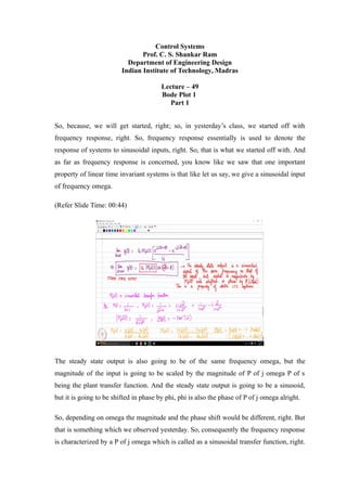
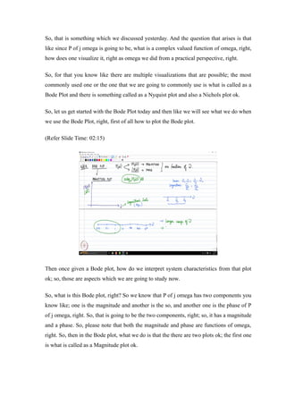
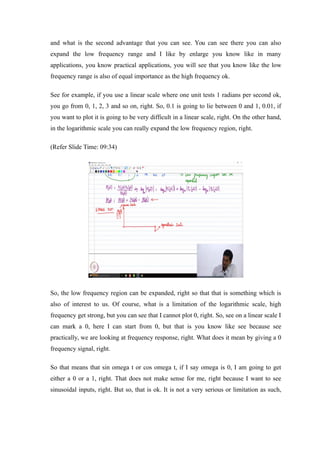
The document discusses Bode plots, which are used to visualize the frequency response of linear time-invariant systems. It begins by reviewing frequency response and how it characterizes the steady-state output of a system to a sinusoidal input. It then introduces Bode plots, which have two components - a magnitude plot and a phase plot. The magnitude plot uses logarithmic scales for both frequency and magnitude in decibels. The phase plot uses a logarithmic scale for frequency and a linear scale for phase in degrees. Using logarithmic scales allows visualization of a wide range of frequencies and magnitudes on the same plot. 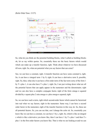The document outlines common building blocks that comprise transfer functions, such as constants, integrals, derivatives, and

1. Control Systems
Prof. C. S. Shankar Ram
Department of Engineering Design
Indian Institute of Technology, Madras
Lecture – 49
Bode Plot 1
Part 1
So, because, we will get started, right; so, in yesterday’s class, we started off with
frequency response, right. So, frequency response essentially is used to denote the
response of systems to sinusoidal inputs, right. So, that is what we started off with. And
as far as frequency response is concerned, you know like we saw that one important
property of linear time invariant systems is that like let us say, we give a sinusoidal input
of frequency omega.
(Refer Slide Time: 00:44)
The steady state output is also going to be of the same frequency omega, but the
magnitude of the input is going to be scaled by the magnitude of P of j omega P of s
being the plant transfer function. And the steady state output is going to be a sinusoid,
but it is going to be shifted in phase by phi, phi is also the phase of P of j omega alright.
So, depending on omega the magnitude and the phase shift would be different, right. But
that is something which we observed yesterday. So, consequently the frequency response
is characterized by a P of j omega which is called as a sinusoidal transfer function, right.

2. So, that is something which we discussed yesterday. And the question that arises is that
like since P of j omega is going to be, what is a complex valued function of omega, right,
how does one visualize it, right as omega we did from a practical perspective, right.
So, for that you know like there are multiple visualizations that are possible; the most
commonly used one or the one that we are going to commonly use is what is called as a
Bode Plot and there is something called as a Nyquist plot and also a Nichols plot ok.
So, let us get started with the Bode Plot today and then like we will see what we do when
we use the Bode Plot, right, first of all how to plot the Bode plot.
(Refer Slide Time: 02:15)
Then once given a Bode plot, how do we interpret system characteristics from that plot
ok; so, those are aspects which we are going to study now.
So, what is this Bode plot, right? So we know that P of j omega has two components you
know like; one is the magnitude and another is the so, and another one is the phase of P
of j omega, right. So, that is going to be the two components, right; so, it has a magnitude
and a phase. So, please note that both the magnitude and phase are functions of omega,
right. So, then in the Bode plot, what we do is that the there are two plots ok; the first one
is what is called as a Magnitude plot ok.

3. So, what is this magnitude plot? In the magnitude plot, we plot omega on the abscissa
and the magnitude of P of j omega on the in the ordinate ok, but the important thing to
note is that like we use a logarithmic scale for omega on the abscissa ok, was the
horizontal axis and this P of j omega is plotted in decibel measure, right.
So, how do we get the decibel measure? So, given a P of j omega, you know like we take
its magnitude and then we take the logarithm to the base 10 and then multiply it by 20
ok, to get the equivalent magnitude and decibel units ok. So, that is what we do ok.
So, now, the question arises you know like why do we do this, right. So, what do you
think is the difference between a logarithmic scale and a linear scale? You know like see
most offers are exposed to a linear scale, right while plotting, right. So, what is a
logarithmic scale? Let us say if I use omega what I say on the; if I plot omega on the x
axis using a logarithmic scale, right how can I characterize it now?
Let us say, you know like I have three points, right. So, let us say you know like I have
omega 2, omega 1, omega 3, right. So, which are, so, the distance between omega 1 and
omega 2 is the same as the distance between omega 2 and omega 3. So, now, if I use a
linear scale, you know like what can I say about the distance between these two sets of
points? They are equidistance, but what does it characterize?
Student: (Refer Time: 05:32) one of them is 10 times.
One of them is.
Student: 10 times the other.
10 times, no if I use a linear scale linear scale, if these 3 points are equidistant from one
another; that is omega 1, the distance between omega and omega 2 is equal to the
distance between omega 2 and omega 3, what does it mean?
Student: (Refer Time: 05:52)
So, if I use a linear scale, right. So, what it means is that omega 2 minus omega 1 is
going to be equal to omega 3 minus omega 2, right. On the other hand, if I use a
logarithmic scale, what can I interpret?

4. Student: Omega 2 by omega 1.
So, these are equidistant, right; so, that distances are equal. So, if I use a logarithmic
scale, the ratios are going to be the same, right. So, if you use a logarithmic scale, omega
2 by omega 1 is going to be equal to omega 3 by omega 2, right.
So, now, on what to say the, if the Bode plot in the x axis or the abscissa, right, so, we
essentially use a logarithmic scale you know like of course, we use a to the base 10,
right. And then, what happens is it if I have what to say 3 points which are equidistant
from one other, this property is going to hold ok. And as he told you know like if you
have you know like a point I want to say essentially 2 points, you know like in a certain
sense you know like we will plot it you know like we will say that you know, one point
is 10 times the previous one and that is how we will define what is called as a decade,
right.
So, we will come to that shortly so. But then, why do we use a logarithmic scale, you
know like why do you think you know like one should use a logarithmic scale instead of
a linear scale.
Student: We can cover vast omega.
Sorry.
Student: If there is too much variation with the omega. The variation of mod of (Refer
Time: 07:43) omega is not (Refer Time: 07:51).
Yes, one point is that like you can essentially plot a wide range of omega, right. See for
example, you know like if I use a logarithmic scale, let us say you know like I want to
plot omega ok, what I can do is that like I can start with let us say a 0.01 ok, I can call
this 0.1, I can call this 10, I can oh sorry 1, 10, 100, let us say a 1000, you get the point,
right. So, and then I can go to 10000 and so on, right.
So, you can see that you know like in a in a fine I want to say in a finite scale I can cover
a vast range of omega, right or the same time you know like if I use a linear scale, you
know it is going to be really difficult, right. So, essentially to plot such a vast scale and
more importantly, you can, so, the first thing is in you can cover a larger range of omega

5. and what is the second advantage that you can see. You can see there you can also
expand the low frequency range and I like by enlarge you know like in many
applications, you know practical applications, you will see that you know like the low
frequency range is also of equal importance as the high frequency ok.
See for example, if you use a linear scale where one unit tests 1 radians per second ok,
you go from 0, 1, 2, 3 and so on, right. So, 0.1 is going to lie between 0 and 1, 0.01, if
you want to plot it is going to be very difficult in a linear scale, right. On the other hand,
in the logarithmic scale you can really expand the low frequency region, right.
(Refer Slide Time: 09:34)
So, the low frequency region can be expanded, right so that that is something which is
also of interest to us. Of course, what is a limitation of the logarithmic scale, high
frequency get strong, but you can see that I cannot plot 0, right. So, see on a linear scale I
can mark a 0, here I can start from 0, but that is you know like see because see
practically, we are looking at frequency response, right. What does it mean by giving a 0
frequency signal, right.
So that means that sin omega t or cos omega t, if I say omega is 0, I am going to get
either a 0 or a 1, right. That does not make sense for me, right because I want to see
sinusoidal inputs, right. But so, that is ok. It is not a very serious or limitation as such,

6. right as far as a logarithmic scale is concerned. So, that is why, we have we use a
logarithmic scale on the abscissa for the frequency.
Now, comes the second question as to why we use a decibel scale for the magnitude
because we take the magnitude, right. We take the logarithm to the base 10 and multiply
it by 20 and converted to decibels, right. Why should I use a logarithmic scale for the
magnitude; same reason, right similar reasons would apply, right. So, I can cover a larger
range of magnitudes in a finite scale correct; see the plant transfer function can have a
wide range of magnitudes.
So, I can have cover a larger range. I can focus on lower magnitude values also right that
region is also going to be expanded. So, can you also like sense any other advantage you
know of using a logarithmic scale.
Let us say if P of j omega, let us say is P 1 j omega times P 2 j omega divided by P 3 j
omega, let us say P 1, P 2 or some factors, right. So, what happens if you use a
logarithmic scale? So, if you then do log of P of j omega, what happens is in of course, to
the base ten. So, we are just going to get log to the base 10 P 1 j omega plus log to the
base 10, sorry this is going to be the magnitude ok, log to the base 10 magnitude of P 2 j
omega minus log to the base 10 magnitude of P 3 j omega, right that is what we are
going to get.
So, consequently you can immediately observe that the, if you have a basically product
and ratios of factors, right. So, what you are going to get is that like once you take the
logarithm, they become the algebraic sum, right of the individual factors. So, that that is
a pretty good advantage which would exploit, right, so, we will see that you give me a
transfer function, I break it into smaller terms what I do is that I plot the magnitude plot
of the individual terms. Then I just add or subtract like as the case may be alright. So,
that that way you know like I can plot the Bode Plots pretty easily ok; we are going to
see how that is going to help us shortly.
Similarly, you can see that the phase of P of j omega is also going to follow a same a
similar what you say trend, right. So, you are we will see that it is going to be phase of P
1 j omega phase of P 2 j omega minus phase of P 3 j omega, right.

7. So, essentially, if you can divide they are basically break down a given transfer function
into simpler building blocks which we are going to look at, then what we do is that like
we just plot the bode diagrams of the individual blocks and then take the algebraic sum
ok, that is it ok. So, then we are done, right. So, that is a very what we say good
advantage of using a logarithmic scale, right even for the magnitude.
So, now, the second plot is what is called as a Phase Plot ok. So, this Bode Plot has two
plots ok. First is the Magnitude Plot ok, second is the Phase Plot. So, what is the Phase
Plot? If the phase plot once again omega is plotted on the abscissa. So, using a
logarithmic scale and the phase of P of j omega is this plotted in degrees using a linear
scale ok. Here, we just use a linear scale like there is no log no need for any logarithmic
scale here ok, you calculate the phase. So, anyway phase of the complex valued function
satisfies this property, right.
So, we do not need to take logarithm assets ok. We just use a linear scale for that ok. So,
that is what the phase plot essentially would visualize, right. So, essentially, the what
happens is that the Bode Plot has two plots, the Magnitude Plot and the Phase Plot. The
Magnitude Plot essentially, plots the magnitude of the transfer sinusoidal transfer
function in decibels versus omega on the x axis or the abscissa using a logarithmic scale.
And the Phase Plot plots the phase of that sinusoidal transfer function in degrees versus
omega once again on a logarithmic scale on the abscissa ok. So, that is what happens
with the Bode Plot, right.
So, as I just discussed you know like one advantage of doing this way is that like, you
can really use certain building blocks if we learn how to plot the bode diagram for the
building blocks, it is easy to plot it for any particular transfer function, right.

8. (Refer Slide Time: 15:57)
So, what do you think are the potential building blocks, what I called as building blocks
ok, let us say within quotes. So, essentially these are the basic factors which would
which can make up a transfer function, right. Think about whatever we have discussed
till now, right. So, what are potential what you say factors that can come?
See, we can have a constant, right. A transfer function can have some constant k, right.
So, it can have a integral term 1 by S, right. It can have a derivative term S, possible,
right. So, then, what else it can have a first order term of the fact term sorry of the form 1
by T s plus 1, it can also have T s plus 1, right. So, I am just writing down what are all
the potential factors that can apply appear in the numerator and the denominator, right
and we can also have a complex conjugate factor, right of the form omega n squared
divided by s square plus 2 zeta omega n s plus omega n squared, right.
So, we can have such a term, right which second-order factor which cannot be factorized
into real what we say factors, right in the numerator. Same way, I can have a second
order factor in the numerator, right of the transfer function in this way ok. So, these are
all potential factors. So, you can see that, can I change the color ok. So, essentially you
know like we can have a constant, we can have 1 by s, right. So, which is like an integral
s which is like a derivative you know like, then I can have 1 by T s plus 1 and then T s
plus 1 in the first order factors you know like. That is what we are looking at and we can

9. have second order factors with complex conjugate roots of this form both in the
denominator on the numerator, right.
So, we can have all these factors, right. So, now, you can immediately observe that, I can
essentially rewrite any transfer function in this particular form. We will see how to do
that, right as we go along, right so, but these are the basic building blocks that we are
going to look at. So, if we understand how to plot the, bode diagram for each of these
building blocks, then we are done, right. So, that is what we are going to look at ok.
So, let us let us understand how to plot the, bode diagram for these blocks ok. So, let me
start from the first block. So, let me consider, of course, I am let me use the term symbol
G of s to say that it is any generic transfer complex valued function ok. So, anyway, K is
a real number. So, of course, K is greater than 0, otherwise I can take logarithm, right.
So, let us say you know the K is greater than 0 and then like we essentially look at this
one ok. So, now, what happens if I want to plot the bode diagram if G of s is k, G of j
omega is going to be just K, right. So, that is it ok. So, then a what will happen? The
magnitude of G of j omega is going to be equal to 20 log to the base 10 magnitude of K
which is just K in decibels ok. So, or of course, k need not be let us let us put a generic
case ok, let us say k k is some real number ok. So, right let us let us do this, right.
Student: So, so we have not called T s plus T s plus 1 instead of doing when there is on
other (Refer Time: 20:12).
I did not get you, I am sorry.
Student: We have covered T s plus 1. Instead of one that (Refer Time: 20:15).
Absolutely, we are going to see how to rewrite ok. That is something which I am going
to show you, right ok; good point. He is saying, why do not you consider 1 by s plus a
for example, you can have factors like this you know like how come, you are making the
constant term as 1 ok, you can see that you can always rewrite a given transfer function
in this form I am going to show it to.
You first let us learn the building blocks, then we will we will do examples, right. So,
where you can easily rewrite in this form, right; so, let us say we essentially take k to be

10. some real number. So, G of j omega is going to be k and magnitude of G of j omega is
going to be 20 log to the absolute value of k in decibels. What can you say about the
phase of G of j omega? It is going to be 0 degrees if k is greater than 0. It is going to be
180 degrees if k is less than 0, right why because if I essentially plot the complex plane
ok, what I call as a G of s plane because I am plotting this factor.
So, let us say you know like if I have K to be positive, you can really see that the phase is
0, right. On the other hand if let us say you know I consider a K 2 which is negative, you
can immediately see that the phase is going to be 180 degrees, right. So, it really depends
on the sign of K ok. So, now, if I want to draw the magnitude plot on the phase plot,
what is it that I should do? So, you can see that, if I draw the magnitude plot on the phase
plot. So, I plot it in decibels and the phase plot also in decibels sorry, the phase plot also
where the phase is in degrees ok. So, what is going to happen to the magnitude plot? The
magnitude plot, you know like I will just have a straight line with respect to omega. That
is it, right. So, where are this value is going to be 20 log to the base 10 of k correct.
So, in the phase plot, I will have either 0 if k is less than 0 or say typically or what we do
is that like we take a negative value we will see why we do that ok. So, we take it as
minus 180 ok. So, typically we will take it as minus 180 if k is less than 0, I will explain
why we take the negative value here ok. So, later on fine.
Student: (Refer Time: 23:14) magnitude of G of j omega as equal to (Refer Time: 23:18).
Yeah so that is there in decibel units.
Student: (Refer Time: 23:23) table equal.
It is basically, it is understood that you know like you are writing in decibels or if you
want to be very particular if you say 20 log to the base 10 magnitude of G of j omega is
fine. So, I got a point. So, let us say I write the magnitude of G of j omega as absolute
value of k. So, then the 20 log to the base 10 magnitude of G j omega in decibels is going
to be 20 log to the base 10 absolute value of K fine ok.
So, that is going to be the Bode Plot for this one, right this constant term. And see,
typically what happens is it like.

11. (Refer Slide Time: 24:03)
We take frequency ranges on the abscissa which are typically. Here it does not matter,
but we essentially use you know like what is called as a decade ok, by convention you
know like we plot frequencies or we mark frequencies, which are a decade apart, right.
What is a decade of frequency? See, a decade essentially means that you are at a
particular frequency you are considering a range from that frequency to either 10 times
that frequency or 0.1 times that frequency ok.
So, let us say what is a decade, at a given frequency omega ok, the range omega to 10
omega is one decade above omega ok. Similarly, the range 0.1 omega to omega is called
as one decade below omega ok. So, that is the definition of this. So, typically, by and
large you know like, we will plot frequencies I would say will mark on the x axis you
know like as Decades ok.
So, you can see that if you consider one as the base frequency, right the frequency under
consideration 10 is one decade above what ok. So, the reason 1 to 10 is a region, one
decade ago 1, right from 0.1 to 1 is one decade below 1 ok. So, that is what this is ok. So,
of course, this is a; I will say a frequency range, right. So, 10 omega is going to be one
decade above omega ok. So, oops sorry I have to be very correct. So, 10 omega is going
to be a one, but typically it is illustrated as a range.

12. So, let me keep it this way, right. So, what do you get the point? So, if you essentially
consider a frequency omega 10 omega is one decade above omega and 0.1 omega is one
decade below omega. By and large it is considered as a range, right.