control systems nptel lecture 1

1. Control Systems
Prof. C. S. Shankar Ram
Department of Engineering Design
Indian Institute of Technology, Madras
Lecture – 01
Introduction to Control Systems
Part - 1
Greetings, welcome to this course on Control Systems; this is a course on control
systems.
(Refer Slide Time: 00:26)
And to be more specific, this is a first level undergraduate course on control systems
where we are going to learn the basics behind what is called as classical control theory.
And we would learn how to design controllers for dynamic systems that we encounter in
practice.
Before we go into the details of what we would learn in this particular course, let us just
look at the title of this course. There are two words in this title. The first word is what we
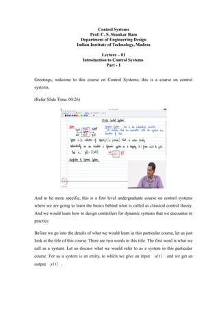
call as a system. Let us discuss what we would refer to as a system in this particular
course. For us a system is an entity, to which we give an input u(t) and we get an
output y(t) .

2. This is typically called as a Dynamic System, it essentially deals with variables, inputs
and outputs that are functions of time. So, as far as this dynamic system is concerned,
time is the independent variable; and all other variables that are associated with the
system are functions of time.
We are going to deal with the so called dynamic systems, where variables change with
time. And a system or a process or a plant is an entity that is given an input and produces
an output. That is the visualization we would be having for the system. There are
alternative terms for the system, some would call the system as a plant.
If you go to chemical engineering, for example, they would be dealing with the
processes, so a process is also visualized as an entity to which we give an input and we
get an output. So, there are various terms that are typically used. For us, a system is a
collection of objects, let us group it as one phrase, a process and that is understood. That
is what we would refer to as a system.
Although we are not going to repeatedly use various adjectives to denote the type of
systems that we are going to look at. We will first study what class of systems that we are
going to be concentrating on and then we will go forward.
The class of dynamic systems that we would be looking at in this particular course
belong to what are called as linear time invariant causal dynamic systems, and by and
large we will restrict ourselves to what are called single input single output systems. So,
before we get into that, we would see that mathematically we can visualize a dynamic
system as a mapping S() from u(t) to y(t) . So, what we are going to say is
that, we have y (t )=S(u(t )) .
So, essentially we would picturize a system as a mapping S() which takes an input
u(t) and delivers an output y(t) . That is a mathematical visualization of a
dynamic system. Given this there are various classes of systems that one could
essentially study. So, let us look at some classes of Dynamic Systems.
(Refer Slide Time: 06:24)

3. As far as classification of dynamic systems is concerned; the first classification that we
would consider is based on the number of inputs and outputs, what we abbreviate as
SISO and MIMO. SISO is nothing but Single Input Single Output, and the abbreviation
MIMO stands for Multiple Input Multiple Output systems.
We can visualize, the input and the output as a mapping from the time domain to the
domain of real numbers. For example, if I deal with a single input single output system, I
can say even the input u(t) is a mapping from the field of real numbers to the field of
real numbers. Because t belongs to the field of a real numbers. Essentially, we take
time and the input is a function of time and in the case of a single input single output
system the input u(t) is a scalar valued function of time.
So, u(t) would be a scalar valued function of time. So, that is why we write it in this
form. And similarly the output y(t) is also a scalar valued function of time. So, that is
a single input single output system. On the other hand, let us say we have, M inputs and
P outputs with the M > 1 and also P > 1.
What is going to happen is that; we have input to be a vector valued function which will
take time and then map it to a vector of dimension M. Similarly, we have the output
vector to be a vector valued function of time which will map it to a vector of dimension
P. So, that will be a scenario of multiple input multiple output system.
In this particular course we are going to be interested in SISO systems, SISO dynamic
systems. So, the first classification was based on the number of inputs and outputs. The

4. second classification that we are going to look at is whether a particular a system is
linear or non-linear.
(Refer Slide Time: 09:33)
Let us look at the definition of linearity shortly. Let us say we have a system S() and
let us say we provide an input u1(t) and we get an output y1(t) . And to the same
system and let us say we provide an input u2(t) and we get an output y2(t) .
Condition 1: Now, given these two arbitrary input output combinations, the question that
we ask ourselves is that; if, to the system, we provide an input that is the sum of these
two arbitrary inputs u1 (t )+u2(t) and if the output is also the sum of the two individual
outputs y1(t )∧y2(t) corresponding to u1(t) and u2(t) .
Condition 2: And if we give any input which is an arbitrary scalar multiple of any
arbitrary input u1(t) , and if the output is the same scalar multiple of the
corresponding output y1(t) .
Then the system is said to be a linear one, provided these two conditions are satisfied,
(condition 1 and condition 2). The first condition what is typically referred to as,
additivity the second condition is referred to as homogeneity. The same definition is the
definition of a linear system, it can be re written in this way; if we have a system S()
and we provide an input which is any arbitrary linear combination of u1(t) and

5. u2(t) ; that means providing a input like c1u1(t )+c2 u2(t) where c1 and c2
are two real numbers.
The question is, whether we get the same linear combination of the two corresponding
outputs y1(t) and y2(t) . If this holds true then the system is linear. These are two
alternative and equivalent ways of defining a linear system, typically people call the
second one as the principle of superposition.
We would see in reality that most processes, most plants, most systems are going to be
non-linear. Linearity, we would realize when we work with practical problems is that, it
is going to be an approximation of reality. This should be kept in mind. In this particular
course we are going to deal with linear systems.
Later, we will go through all the classifications and summarize what we are going to deal
with. The third classification that we are going to look at is that of a time invariant
system versus a time varying system. The question is that, what is this concept of time
invariance. Let us demonstrate by a simple diagram. So, let us say we have a system and
we provide some input u(t) to it at time t=0 , let us say we provide a step input.
And we get an output. Now let us say, we now provide the same input u(t) after a
time interval of T . The question becomes do we get the same output. If the output is
the same function which is delayed by T, then the system is said to be time invariant or in
other words the question that we are asking ourselves is that, do we get the same output;
if we provide the same input no matter at what time we provide the input to the system, if
that is the case then the system is said to be time invariant.

6. (Refer Slide Time: 15:56)
A time invariant system is one that provides the same output for the same input
irrespective of when the input is given. For example, we take the example of a ceiling
fan, that most of us encounter every day.
Suppose, if I come and switch on a ceiling fan, I am providing an electrical signal as an
input to the system. And let us say the output of the system is the rpm of the fan, the
speed of rotation of the fan. So, I switch on the fan today, and I give some electrical input
to the fan. And let us say the speed of the fan is, 100 rpm.
And I come tomorrow and switch on the same fan, provided the electrical input is the
same, I would expect the speed to be close to 100 rpm once again. Now if I come after a
month and switch on the same fan there may be some wear and tear in the fan. Given the
same electrical input signal, I may get the rpm as 99.5.
If I come one year down the line and switch on the same fan, giving the same electrical
input signal the rpm may be 99 rpm. For all systems dynamic characteristics change with
time, due to various factors. In the case of a fan there may be some wear and tear, the
components might have become old, then the systems response changes.
Now, the question that we are asking ourselves is that in the time scale of interest, as far
as systems analysis is concerned, do that response characteristics of the system remain
more or less the same. If that is the case, then we approximate the system as a time

7. invariant system. In the case of a fan, let us say I want to analyze the fan only for a few
minutes.
In those few minutes I can reasonably assume that the response characteristic of the fan
is not going to change. What do I mean by that? In a timescale of a few minutes if I
provide the same electrical signal at any instant of time I am going to get close to 100
rpm. Which is what I started off here. On the other hand, if I use a fan in an industrial
application where it is supposed to run for months without any shutdown then I need to
be a bit more careful.
But then my timescale of interest goes in the order of months. So, then we need to ask
ourselves the question, do I need to consider the variation in the systems response
characteristics and model the system as a time varying system. So, there is a question
which should be considered, asked then. In our course, we would work with what are
called time invariant systems. That is the scope of our particular course.
As far as we are concerned, what is the mathematical definition of time invariant
systems; if y(t) is S(u(t )) then time invariance implies that
S (u(t−T))=y(t−T) , for all T belonging to the field of real numbers. In essence, if I
shift the input by a time of T, I should get the same output shifted by the same amount of
time. That is what time invariance means.
In this particular course we are going to work with time invariant systems. Once again
time invariance is an approximation. I am sure all of us agree that if you look at
processes and systems that surround us you will see that no system provides the same
output, at any point of time in it is entire lifetime right. So, time variance may become
important.
But the question we need to ask ourselves is that: what is the time scale of interest to be
serviced, the time scale over which the systems characteristics change, when we decide
to approximate something as time invariant or time varying.
Another classification that we are going to do is that of causal systems versus non causal
systems. What is a causal system? A causal system is one where the output at any instant
of time depends only on past and current inputs. A causal system is one in effect, that is

8. non anticipative, It does not try to figure out what inputs may come to the system in the
near future and take action right now.
(Refer Slide Time: 22:37)
A causal system is non anticipative, whereas a non-causal system is anticipative.
In this particular course we are going to consider systems that are causal. Let us recall
where we really started off and what we are doing in this particular course. We started off
with the title of this course. The first word we started off looking at is the word
SYSTEMS.
We are going to look at what are called DYNAMIC SYSTEMS. We are going to look at
CAUSAL SYSTEMS. We are going to look at TIME INVARIANT SYSTEMS. We are
going to look at LINEAR SYSTEMS and we are going to look at SINGLE INPUT
SINGLE OUTPUT SYSTEMS.
This is the class of systems that will be under study in this course. We are going to
consider SISO LINEAR TIME INVARIANT CAUSAL DYNAMIC SYSTEMS. I hope
through this discussion it is clear as to what each one of these words mean.
By and large linear time invariant is abbreviated as LTI. Typically, LTV stands for Linear
Time Varying systems. Of course, when I ask the question is this a reasonable class of
systems to study; the answer is yes. This is a useful class of systems to study because we

9. will see that, when we later look at case studies and so on, this is a reasonable
approximation as far as many practical problems are concerned.
Now, having looked at the word system now we come to the word Control. What is
control? The word control essentially means making a system behave as design. That in a
very generic sense is what we would refer to as control.
Now, the questions are how we regulate the system. That is something which we are
going to look at. Let us look at an example, armature control of a DC motor. I provide a
voltage v(t ) to the DC motor and the shaft speed ω(t) is output of the DC motor.
I visualize the DC motor as a system to which I provide a voltage input v(t ) , and get
the speed output ω(t) . Now the question when we want to design controller is that; if
I want to maintain the speed of the DC motors output shaft at a particular value, what
voltage input do I need to provide. If we wish to achieve ωd , desired angular speed
for the DC motor, what is the input voltage that should be provided. This whole course
about a learning how do we do this process, which is the idea behind this.
In a general sense, we are going to learn how to design controllers, for many practical
systems, that belong to the class of interest.
What is our approach that we are going to follow? In a very generic sense, we are first
going to develop a mathematical representation for S() . That is the first step. S()
is the mapping between the input and output, and we follow this process to get a
mapping for S() .

10. (Refer Slide Time: 30:16)
This typically constitutes what is called as a mathematical modeling for the dynamic
systems. There can be various ways of obtaining these mathematical models. In this
particular course we would employ physics based models; of course, we can also have a
data driven models or empirical models and sometimes we use both.
We use physics to essentially derive part of the model, and a part of the model is
obtained by using experimental data. There can be a semi empirical approach also. First
step is to essentially develop a mathematical representation for the mapping S() and
then second step is to analyze the system response. And then the third step is essentially
to design the controller.
So, in a very broad sense, a big picture view perspective, these are the three steps
involved in our approach, which we are going to learn in this particular course. There are
also various categories of models we will see.