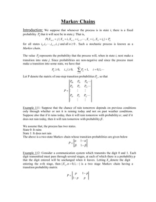
This document introduces Markov chains and provides examples to illustrate key concepts. Markov chains model stochastic processes where the probability of transitioning to the next state depends only on the current state, not on the process history. The document defines one-step and n-step transition probabilities and the Chapman-Kolmogorov equations for computing n-step probabilities. Examples include weather modeling, communication systems, and gambling.

1. Markov Chains
Introduction: We suppose that whenever the process is in state i, there is a fixed
probability ijP that it will next be in state j. That is,
1 1 1 1 1 0 0( | , , , , }n n n n ijP X j X i X i X i X i P       
for all states 0 1 1, , , , , and all 0ni i i i j n  . Such a stochastic process is known as a
Markov chain.
The value ijP represents the probability that the process will, when in state i, next make a
transition into state j. Since probabilities are non-negative and since the process must
make a transition into some state, we have that
0
0, , 0; 1, 0,1,ij ij
j
P i j P i


    
Let P denote the matrix of one-step transition probabilities ijP , so that
00 01 02
10 11 12
0 1 2i i i
P P P
P P P
P
P P P



  

  
We assume that, the process has two states.
State 0: It rains
State 1: It does not rain
The above is a two-state Markov chain whose transition probabilities are given below
1
1
P
 
 



1
1
p p
P
p p



Example 111: Suppose that the chance of rain tomorrow depends on previous conditions
only through whether or not it is raining today and not on past weather conditions.
Suppose also that if it rains today, then it will rain tomorrow with probability ; and if it
does not rain today, then it will rain tomorrow with probability  .
Example 112: Consider a communication system which transmits the digit 0 and 1. Each
digit transmitted must pass through several stages, at each of which there is a probability p
that the digit entered will be unchanged when it leaves. Letting Xn denote the digit
entering the n-th stage, then {Xn ,n  0,1,} is a two stage Markov chain having a
transition probability matrix P00 = Bit entered stage as 0 and left stage as 0 (no error)
P01 = Bit entered stage as 0 and left stage as 1 (error!!!)
P11 = Bit entered stage as 1 and left stage as 1 (no error)
P10 = Bit entered stage as 1 and left stage as 0 (error!!!)
In Simple words, if the next state Xn+1 depends only on current state Xn and
NOT on any other prior state (i.e., Xn+1 is NOT dependant on Xn-1, Xn-2, ... X0) then
the process can be modelled as a Markov Chain
Transition Probability
Matrix

2. 0.5 0.4 0.1
0.3 0.4 0.3
0.2 0.3 0.5
P 
Transforming Process into Markov Chain: Suppose that, whether or not, it rains today
depends on previous weather conditions through the last two days. Specially suppose that
if it has rained for the past two days, then it will rain tomorrow with probability 0.7; if it
rained today but not yesterday, then it will rain tomorrow with probability 0.5; if it rained
yesterday but not today, then it will rain tomorrow with probability 0.4; if it has not
rained in the past two days, then it will rain tomorrow with probability 0.2.
If we let the state at time n depend only on whether or not it is raining at time n, then the
above model is not a Markov chain. However, we can transform the above model into a
Markov chain by saying that the state at any time is determined by the weather conditions
during both that day and the previous day. That means, we can say that the process is in
State 0: if it rained both today and yesterday
State 1: if it rained today but not yesterday
State 2: if it rained yesterday but not today
State 3: if it did not rain either yesterday or today.
The preceding would then represent a four-state Markov chain having a transition
probability matrix
0.7 0 0.3 0
0.5 0 0.5 0
0 0.4 0 0.6
0 0.2 0 0.8
P 
chain.
State 0: Cheerful (C)
State 1: So-so (S)
State 2: Glum (G)
The transition probability matrix for this three state Markov chain is given below
Example 113: On any given day Gary is either cheerful (C), so-so (S) or glum (G). If he is
cheerful today, then he will be C, S, or G tomorrow with respective probabilities 0.5, 0.4,
0.1. If he is felling so-so today, then he will be C, S or G tomorrow with probabilities 0.3,
0.4, 0.3 respectively. If he is glum today, then he will be C, S or G tomorrow with
probabilities 0.2, 0.3, 0.5.
Let, Xn denote Gary’s mood on the n-th day, then {Xn ,n  0}is a three state Markov
Today's Today is Tomorrow's Yesterday
Today's "Today" is Tomorrow's "Yesterday"
P01 ==>(yT=0) => (Tt=1)
y = yesterday
T = Today
t = Tomorrow
*See Last Page Attached*
(Also, Build the matrix if data given in this manner (columnwise):
If he is cheerful, so-so or gloom today, then tomorrow he will be cheerful with
probability 0.5, 0.3, 0.2, so-so with probability 0.4, 0.4, 0.3 and gloom with
probability 0.1, 0.3, 0.5, respectively.)
In each row, one value can be missing,
which you can easily compute
(because row sum always = 1.0
column sum NOT necessary to be 1.0)
Note: here 'not' add korle matrix er value gulo different hoye jabe!!!

3. Random Walk Model: A Markov chain whose state space is given by integers
0, 1, 2,i     is said to be a random walk if, for some number 0 1p  ,
, 1 , 11 , 0, 1, 2,i i i iP p P i       
The preceding Markov chain is called a random walk for we may think of it as being a
model for an individual walking on a straight line who at each point of time either takes
one step to the right with probability p or one step to the left with probability1 p .
A Gambling Model: Consider a gambler who, at each play of the game, either wins $1
with probability p or loses $1 with probability1 p . If we suppose that our gambler quits
playing either when he goes broke or he attains a fortune of $N, then the gambler’s
fortune is a Markov chain having transition probabilities
, 1 , 1
0,0 ,
1 , 1,2, , 1
1
i i i i
N N
P p P i N
P P
     
 

Sate 0 and N are called absorbing state since once entered they are never left. Note that
the above is a finite state random walk with absorbing barriers (Sate 0 and N).
Chapman-Kolmogorov Equation: We have already defined one-step transition
probabilities ijP . We now define the n-step transition probabilities n
ijP to be the probability
that a process in state i will be in state j after n additional transitions. That is,
{ | }, 0, , 0n
ij n m mP P X j X i n i j    
The Chapman-Kolmogorov equations provide a method for computing these n-step
transition probabilities. These equations are
0
for all , 0, all ,n m n m
ij ik kj
k
P P P n m i j



 
days from today given that it is raining today.
Solution: The one-step transition probability matrix is given by
0.7 0.3
0.4 0.6
P 
Hence,
2 0.7 0.3 0.7 0.3
0.4 0.6 0.4 0.6
0.61 0.39
0.52 0.48
P P P   

n-step transition matrix may be obtained by multiplying the matrix P by itself n times.
Example 114: Consider Example 1, in which the weather is considered as a two-state
Markov chain. If  0.7 and   0.4 , then calculate the probability that it will rain four

4. 4 2 2 0.61 0.39 0.61 0.39
0.52 0.48 0.52 0.48
0.5749 0.4251
0.5668 0.4332
P P P   

and the desired probability 4
00P equals 0.5749. (Ans.)
2
0.7 0 0.3 0 0.7 0 0.3 0
0.5 0 0.5 0 0.5 0 0.5 0
0 0.4 0 0.6 0 0.4 0 0.6
0 0.2 0 0.8 0
P P P   
0.2 0 0.8
0.49 0.12 0.21 0.18
0.35 0.20 0.15 0.30
0.20 0.12 0.20 0.48
0.10 0.16 0.10 0.64

Since rain on Thursday is equivalent to the process being in either state 0 or sate 1 on
Thursday, the desired probability is given by 2 2
00 01 0.49 0.12 0.61P P    (Ans.)
☺Good Luck☺
Example 115: Consider Example in Page 2. Given that it rained on Monday and
Tuesday, what is the probability that it will rain on Thursday?
Solution: The two-step transition matrix is given by
State 0 = Rained THU & Wed
State 1 = Rained THU, but Not Wed
What is probability it will Rain on Thu, but not
on Wed? (Ans: P^2 Matrix er value of index 01)
OR, (P^2)01 = 0.12
It is NOT (P00)^4, Rather it is (P^4)00
So, Find the P^4 Matrix at first
(P^2)ij
j: State 0 = Rained Today & Yesterday
State 1= Rained Today, but NOT yesterday
What is the Probability that it Won't Rain of Thursday given it Rained on Mon & Tuesday?
Ans: (P^2)02 + (P^2)03
What is the Probability that it will Rain of Thursday given it Rained Neither on Monday Nor
onTuesday?
Ans: (P^2)30 + (P^2)31
What is the Probability that GARY will be cheerful after FOUR days given that he is Gloom today?
Ans: (P^4)20
What is the Probability that GARY will NOT be cheerful after FOUR days given that he is Gloom today?
Ans: 1 - (P^4)20 OR { (P^4)21 + (P^4)22 }
What is the Probability that GARY will be cheerful after FOUR days given that he is Cheerful today?
Ans: (P^4)00
(it does NOT matter whether it Rained or Not at the intermediate day = Wednesday)
Probability of Rain after four days given today Not Raining = 0.5668
Probability of No Rain after four days given today Raining = 0.4251 Probability of NO Rain after four days given today Not Raining = 0.4332

5. Today/Monday state = 0
(means Rain on Sun & Mon
Tomorrow/Tuesday state = 0
(means Rain on Mon & Tue)
Today/Monday state = 0
(means Rain on Sun & Mon)
Tomorrow/Tuesday's state = 1
(means Rain on Tue,
but NO rain on Mon)
Today/Monday state = 0
(means Rain on Sun & Mon)
Tomorrow/Tuesday state = 2
(means NO Rain on Tue, but Rain on Mon)
Today/Mon=0 (Rain on Mon+Sun)
Tmrw/Tues=3 (NO Rain Tue+Mon)
it is
.

6. Markov Chains
The Gambler’s Ruin Problem: Consider a gambler who at each play of the game
has probability p of winning one unit and probability 1q p  of losing one unit.
Assuming that successive plays of the game are independent, what is the probability that
starting with i units, the gambler’s fortune will reach N before reaching 0?
If we let nX denote the player’s fortune at time n, then the process{ , 0,1,2, }nX n   is a
Markov chain with transition probabilities
00
, 1 , 1
1
1 , 1,2, , 1
NN
i i i i
P P
P p P i N 
 
    
This Markov chain has three classes namely {0},{1,2, , 1}N  and {N}; the first and
third class being recurrent and the second transient. Since each transient state is visited
only finitely often, it follows that, after some finite amount of time, the gambler will
either attain his goal of N or go broke.
Let , 0,1, ,iP i N  , denote the probability that, starting with i, the gambler’s fortune will
eventually reach N. By conditioning on the outcome of the initial play of the game we
obtain
1 1
1 1
1 1
1 1
1 1
, 1,2, , 1
( )
( ) ( )
( ), 1,2, , 1 (1)
i i i
i i i
i i i i
i i i i
i i i i
P pP qP i N
p q P pP qP
pP qP pP qP
p P P q P P
q
P P P P i N
p
 
 
 
 
 
   
   
   
   
     

 
Hence, since 0 0P  , we obtain from preceding line that
Putting i = 1 in equation (1), we get, 2 1 1 0 1( )
q q
P P P P P
p p
   
Putting i = 2 in equation (1), we get,
2
3 2 2 1 1( )
q q
P P P P P
p p
 
     
 

Putting i = i in equation (1), we get,
1
1 1 2 1( )
i
i i i i
q q
P P P P P
p p

  
 
     
 

Putting i = N in equation (1), we get,
1
1 1 2 1( )
N
N N N N
q q
P P P P P
p p

  
 
     
 
N = Total no. of Coins in the System
= Total no. of Coins of Player1 + Player 2
{as p+q=1}
P4 - P3 = ...
Modelling the Gambler's Ruin Problem: An Example of the Application of Markov Chain
Other Applications of Markov Chain Theory: Modelling Random Walk/Brownian Motion,
Simulating Population Growth or Birth/death process etc.

7. Adding the first 1i  of these equations yields,
2 1
1 1
i
i
q q q
P P P
p p p

      
          
       

2 1
1 1
i
i
q q q
P P
p p p

      
           
       

If 1
q
p
 , then
 
 
2 1
1
1
1
, 1
11
i
n
n
i
q
p x
P P x x x
q x
p

 
   
          
  
 
If 1
q
p
 , then 1 1[1 1 1]i
i
P P iP    
Thus,
 
 
1
1
1
, if 1
1 (2)
, if 1
i
i
q
p q
P
q p
P p
q
iP
p
 
 
 
    




Putting i = N in equation (2), we get,
 
 
1
1
1
, if 1
1 (3)
, if 1
N
N
q
p q
P
q p
P p
q
NP
p
 
 
 
    




Now, using the fact that 1NP  in equation (3), we obtain that
If 1
q
p
 , then
 
 
1
1
1
N
N
q
p
P P
q
p
 
 
  
 
  
 
 
1
1
1
N
q
p
P
q
p
 
 
   
 
  
If 1
q
p
 , then 11 NP
1
1
P
N
 
***
These formulas are OK
even when p < q OR p> q OR p = q
***
Or, p = q = 1/2 Or, p == q (i.e., when winning chance = loosing chance.
example: fair coin toss => head=win, tail = loss
or vice versa)
Partial proof
may appear
in exam !!!

8.  
 1
1
1
if
2
1
1 1
, if
2
N
q
p
p
qP
p
p
N
 
 
 
     



Putting the value of 1P in equation (2), we get
If
1
2
p  , then
 
 
 
 
 
 
1 1 1
1 1 1
i i
i N N
q q q
p p p
P
q q q
p p p
   
     
     
     
      
If
1
2
p  , then
1
i
i
P i
N N
 
Finally, we get
 
 
1
1
, if
2
(4)1
1
, if
2
i
N
i
q
p
p
qP
p
i
p
N




 




Example: Suppose Max and Patty decide to flip pennies; the one coming closest to the
wall wins. Patty, being the better player, has a probability 0.6 of winning on each flip.
(a) If Patty starts with five pennies and Max with ten, then what is the probability that
patty will wipe Max out?
(b) What if Patty starts with ten and Max with twenty?
Solution: (a) Let, 5, 5 10 15, 0.6, 1 1 0.6 0.4i N p q p         
Hence the desired probability is
 
 
5
5 15
0.41
0.6 0.87
0.41
0.6
P

 

(Ans.)
(b) Let, 10, 10 20 30, 0.6, 1 1 0.6 0.4i N p q p         
Hence the desired probability is
 
 
10
10 30
0.41
0.6 0.87
0.41
0.6
P

 

(Ans.)
☺Good Luck☺
p = winning probability (of the person)
q = 1- p = losing probability
i = starting number of coins (of the person)
N = total coins in the system
, q = 1/2 (or, p = q)
This is full proof
Full proof
may appear
in exam, Too!
This is why p = 0.6, q =0.4, i=5 (If we ask "Max will wipe Patty out", then p=0.4, q=0.6, i=10)
Think: How to solve when p = q = 0.5
* Also: see similar questions in the Practise Questions 03.doc *