control systems nptel lecture 4

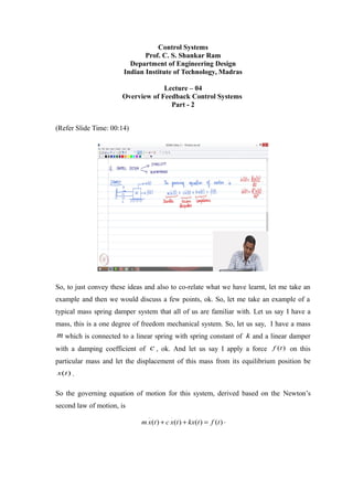
1. Control Systems
Prof. C. S. Shankar Ram
Department of Engineering Design
Indian Institute of Technology, Madras
Lecture – 04
Overview of Feedback Control Systems
Part - 2
(Refer Slide Time: 00:14)
So, to just convey these ideas and also to co-relate what we have learnt, let me take an
example and then we would discuss a few points, ok. So, let me take an example of a
typical mass spring damper system that all of us are familiar with. Let us say I have a
mass, this is a one degree of freedom mechanical system. So, let us say, I have a mass
m which is connected to a linear spring with spring constant of k and a linear damper
with a damping coefficient of c , ok. And let us say I apply a force )(tf on this
particular mass and let the displacement of this mass from its equilibrium position be
)(tx .
So the governing equation of motion for this system, derived based on the Newton’s
second law of motion, is
)()()()(
...
tftkxtxctxm  .

2. Of course, in this particular course if I use a dot over a variable, that means, I am taking
it's time derivative. So, )(
.
tx means it is the first time derivative of )(tx , )(
..
tx means
it is the second derivative of )(tx with respect to time and so on, ok.
So this is the governing equation for this mass spring damper system. As we know,
)(
..
txm characterizes the inertia effects that occur in the system; )(
.
txc corresponds to
the viscous dissipation that happens due to the presence of damper; )(tkx is indicative
of the compliance that is present in the system.
So, these are typically used to visualize this class of mass spring damper systems and
even one would use these analogies to develop models for even other systems from other
domains. So, but let us consider this example and we immediately realize that the
governing equation is a second order linear inhomogeneous ordinary differential
equation with constant coefficients, ok.
(Refer Slide Time: 03:06)
So, we can see that, the order of the system is 2, because we have a second order
derivative, in the governing equation. It is linear as is evident from the governing
equation, because the equation is linear in )(tx and )(tf . It is inhomogeneous because
we have a forcing term on the right hand side of this ordinary differential equation. And
the ODE has constant coefficients which is reflective of the system being time invariant.

3. So, this is essentially an LTI causal single input single output system, ok, the class of
systems that we are essentially looking up.
So, if we look at the response of the system, we are going to have two components, one
due to the presence of any potential non-zero initial conditions and other due to input
provided. So, for example, I can displace the mass a little bit and then leave it, right. So,
then I am giving a non-zero displacement as an initial condition. This would be called as
the free response. And then we can also have a system response, due to the input
provided. In this case, the force is the input to system.
So in fact, if we want to visualize this using the typical systems perspective, in this case
of the mass spring damper system, the input is the force )(tf and the output is the
displacement )(tx . So, in other words, based on the input (force) that is provided I can
have a displacement, right. So, that is what is called as forced response of the system.
The system response can have both components (free and forced response) and this is an
example of a linear time invariant causal SISO system.
On the other hand, let us say, we consider a scenario where the spring constant changes
with time. So, for example, if I keep on operating the system for a long time, the spring
may weaken, right. So, then the spring constant may change with time, right. Let us
consider the scenario where the spring constant changes with time, then the governing
equation could be rewritten as,
)()()()()(
...
tftxtktxctxm 
So, this )(tk is a representative to of a time varying spring constant. A time varying
parameter comes in the system model. So, as a result this becomes what is called as a
linear time varying system. So, this is just an example of when we could potentially get a
linear time varying system instead of a linear time invariant system. We can immediately
realize that the governing equation in this case is once again a second order linear
inhomogeneous ordinary differential equation but with time varying coefficients. So, we
will have time varying coefficients in the governing equation, ok. So, that is something
which will come into play.

4. (Refer Slide Time: 07:45)
Now, let us consider another example. Let us consider a scenario where the spring is
non-linear. This also could be a potential scenario which can be encountered in practice.
So, what do we mean by this. So essentially, in many problems in practice, if we have a
coil spring in some machine element or let us say even in our automotive suspensions,
right. We take a spring and then, we test it by giving force and then plot the force
displacement characteristics.
So, by and large what may happen is that, we may get a curve which may be non-linear,
if we test it in the entire domain, ok. So, what typically happens is the following. Let’s
say in a two wheeler, you know you would have seen a coil spring which essentially
deflects as the two-wheeler is going.
So, let us say we have the spring in an initial state of compression, right. Let us call this
displacement as ix and by and large we would operate the spring in a region around this
ix . It may so happen that the spring may be operated in a region around this initial state,
you know, most of the time. Then, we can immediately observe that in this region the
spring can be approximated as a linear element.
So, then the question that we can ask ourselves is the following, right. Given this range
of operation of the spring, can I use a linear approximation to model the process? If yes, I

5. could use a linearized model and then we can go to the class of linear time invariant
systems. But on the other hand, let us say, I am in an application where the spring is
stretched and compressed over a wide range of displacements, then I may no longer be
able to use a linear model for the spring. Then what is it that I can do?
I am just taking an example, where let us say you know, the governing equation for the
springs response is a quadratic function of the displacement, right. So, what will happen
is that the governing equation for this mass spring damper system will then become
)()()()( 2
...
tftkxtxctxm 
So, you see that the term )(2
tkx makes this system non-linear, ok. So, this becomes a
non-linear system. We could immediately observe that this is still a second order ODE,
but now it becomes a non-linear ODE, right, so, non-linear inhomogeneous ODE with
constant coefficients. So that is what happens to this governing equation, ok.
So, we are just considering different examples to just learn how the governing equations
would change depending on the scenario just to get a broad idea about the class of
systems that we are studying. So, I hope just through the simple example the difference
between linear, non-linear systems and time invariant, time varying systems have
become a little bit clear and we just considered a simple example to show how these
attributes are reflected in the governing equations of such systems, ok. So, to conclude
this class, let me just show you some simple examples just simple simulation results to
convey the concepts what we have learnt.
(Refer Slide Time: 14:19)

6. So, let us consider the mass spring damper system that we have been looking at. Let us
say, I consider these following parameters. I consider the mass of the element to be 1
kilogram, the damping coefficient to be 0.5 Ns/m and the spring constant 0.75 N/m, just
take some values to just solve those equations, right. So, let us say that we provide a
force input of 1 Newton at time t=0.
So, if we solve this mass spring damper system, as we have already discussed, we can
have what is called as the free response of the system, that is we can have non-zero
initial conditions and we have what is called as the free response which is essentially
indicated by this blue curve, right. We can see that the initial displacement is at one and
then it essentially oscillates and then goes to a 0 finally, ok.
On the other hand I can have a zero initial condition and then give an input to the system,
which essentially is what is called as a forced response, right. So, that is the response
term due to the input that we provide and that is denoted by the red curve which
essentially goes and settles down at some non-zero final value, ok. So, if we combine
both that is we give non-zero initial condition and the input we will we get the curve
which is indicated black. So, we can see that the response is the sum of both
contributions, that is the free response plus forced response term gives the third response,
right, where we have a response from that mass spring damper system that consists of
both the non-zero initial condition component and the force input component, right.
So, once again please remember, what our system was. For us the mass spring damper
system was visualized as one to which we give the force as the input and the
displacement is output, ok. That is why we are essentially plotting the displacement and
studying it. So, this is just to show whatever we have learnt through a graphical
visualization.

7. (Refer Slide Time: 16:36)
So, let us now look at time variance. Now, let us say instead of having a constant spring
constant of 0.75 N/m, let us say the spring has a varying spring constant, which is of this
form t
e 001.0
75.0 
N/m. So, the spring constant is slowly decreasing from the initial
value of 0.75, right. So, if we plot it, of course, we can see that I have just zoomed in into
a range of 0 to 100 seconds.
So, may be around the 75th second we can see that the spring constant has decreased to
around 0.693 N/m, ok. So, that is what has happened. So, and as we just discussed a few
minutes back the governing equation now becomes
)()()()()(
...
tftxtktxctxm 
So, this makes it as a linear time varying system, ok. So, we can see that the system has
now, become LTV right, due to this time varying spring constant. So, let us see what
effect of this on the system response is.

8. (Refer Slide Time: 17:57)
So, we consider zero initial conditions and so let us not worry about the free response.
We only look at the force response here. So, what we do is that we are giving an unit step
force input of 1 Newton in one scenario at t=0 which is the response is indicated by the
blue curve and then what we do is that, we then give the same unit step force input at a
time, instant of 75 seconds. So, as we realize from the previous slide, at time t equals 75
seconds the spring constant decreased. So, because this is a time varying parameter in
this particular case, so you could immediately see that the response, which is plotted by
the red curve is different from the blue curve right with this essentially, going against the
definition of time invariance.
So, if you recall the definition of time invariance, if we give the same input at let us say
time t=0 and time t=75, as in this example I should get the same output right, but that is
not the case. Why? Because, we have a time varying system, ok. So we can immediately
see that the red curve is different from the blue curve, right. So, you can see the peak of
these oscillations that has increased in the red curve when compared to the blue curve,
right. So, in, in certain sense, the responses are becoming, different ok. So, this gives us
an overview of how these factors affect the system response. Through simple examples,
I just wanted to communicate how linearity time invariance and all come into play, ok.

9. So, we would stop here. So, we have essentially looked at a big picture view of what we
are going to learn in this particular course and defined a few terms in this particular class
and then looked at an example. That’s what we have done here and we also looked at
what is meant by sensor dynamics, actuator dynamics and unity, non unity feedback and
so on. So, in the next class, we would essentially meet and start off with mathematical
preliminaries and we would revise mathematical tools that we would be using in this
particular course, ok.
Thank you for your attention.