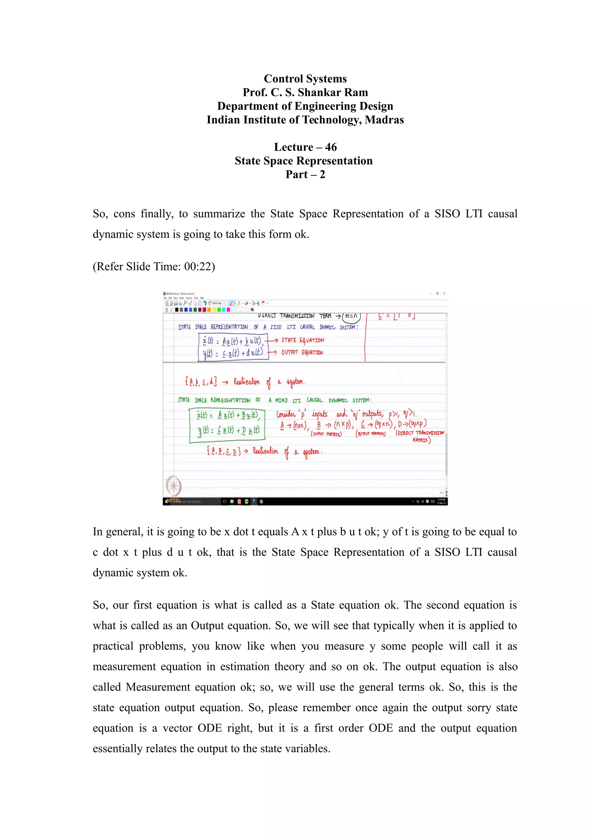
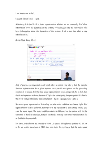
The document discusses the state space representation of linear time-invariant (LTI) systems. It provides the following key points: 1. The state space representation of a single-input single-output (SISO) LTI system is given by x ̇(t) = Ax(t) + bu(t) and y(t) = cx(t) + du(t), where x(t) is the state vector, u(t) is the input, y(t) is the output, and A, b, c, d are matrices that characterize the system. 2. For multiple-input multiple-output systems, u(t) and y(t) become

1. Control Systems
Prof. C. S. Shankar Ram
Department of Engineering Design
Indian Institute of Technology, Madras
Lecture – 46
State Space Representation
Part – 2
So, cons finally, to summarize the State Space Representation of a SISO LTI causal
dynamic system is going to take this form ok.
(Refer Slide Time: 00:22)
In general, it is going to be x dot t equals A x t plus b u t ok; y of t is going to be equal to
c dot x t plus d u t ok, that is the State Space Representation of a SISO LTI causal
dynamic system ok.
So, our first equation is what is called as a State equation ok. The second equation is
what is called as an Output equation. So, we will see that typically when it is applied to
practical problems, you know like when you measure y some people will call it as
measurement equation in estimation theory and so on ok. The output equation is also
called Measurement equation ok; so, we will use the general terms ok. So, this is the
state equation output equation. So, please remember once again the output sorry state
equation is a vector ODE right, but it is a first order ODE and the output equation
essentially relates the output to the state variables.

2. So, you can see what has happened here right. So, in the transfer function representation
of the mass spring damper system what did we do? We directly took the Laplace of the
output to the Laplace or the input as 1 by ms squared plus c s plus k right; you give me
any input; I can directly calculate the output. Here what has happened is that yes, we are
given an input; what we do is that we first solve for the state variables which in a certain
sense characterize the internal dynamics of the system and then get the output from the
state variables ok. So, it is a 2 step process as to what we are doing.
So, for that reason you know like the transfer function representation is also what is
called as an external representation of the system because it directly relates the input and
the output. The state space representation is what is called as a internal representation of
the system or represents what is called as the internal dynamics of the system because we
go through the state vector ok. So, that is what we are doing in the state space
representation.
Student: (Refer Time: 03:30).
State space because you are going to have a vector as a state variable right state varient
vector right; so, you are essentially going to the space of state variables right it is a
vector space ok. So, that is why it is called a state space representation ok. It is a space of
state variables ok; so, that characterizes the system ok.
So and typically the set A, b, c, d is what is called as a realization of a system ok. So, that
is a terminology which we will encounter that is what is called as a realization of a
system fine. So, now similarly the state space representation of a MIMO LTI causal
dynamic system is going to be the following ok.
So, what happens in the case of a multiple input multiple output dynamic system? What
is going to happen is an A x dot t is going to be equal to A x t plus capital B u t ok. Now
u is a vector the matrix, you will still have n state variables; n being order of the system
ok; but the changes the second term which is B u t, B will become a matrix ok. Because
u is a vector and similarly the output equation, since y is a vector we will have it as C x
of t plus D u of t ok.
So, that is the change which will happen.

3. Student: (Refer Time: 05:48).
I am sorry, what is that?
Student: (Refer Time: 05:52).
No, we do not have, but I am just introducing it to you right. So, essentially let us say
consider let say m inputs or let me use a different character, let us say p inputs and q
outputs ok; of course, p q greater than 1 right for a MIMO system ok. So, now, what do
you think will be the size of each of these matrices? The; what to say the state matrix A is
still the state matrix that will be n by n that is not going to change right. Now, B is the
input matrix right. What will be the size of the input matrix?
So, B is now called as an input matrix ok. Ok, previously small b was a called as an input
vector ok. Now, it is called input matrix; what do you think should be the size? It is
going to be equal to n cross p right because you are multiplying a vector of dimension p
right u is a vector of dimension p right because there are p inputs right.
So, then you must have p columns in B and the product gives you a vector x dot; x dot
has n, n is of dimension n right. So, the number of rows in B should be n; so, that is why
we the size of B to be n by p right. Then like C, the matrix C what is it going to be? We
call it as the output matrix ok. What would be the dimension? It is going to be q, q by n
right. So, that is what we are going to get for C and what about the size of D? D is what
is called as the direct transmission matrix what is the size of D now?
Student: (Refer Time: 08:21).
It is going to be q by b; q by right because please note that D is multiplying u right; you
have; you use dimension as p. So, it must have p columns and it is mapped to y which is;
whose dimension is q. So, D must have q rows right.
So, then in the MIMO domain right the matrices A B C D form what is called as a
realization ok. Here, we do not have the issue of notation of C and C transpose ok. So,
the matrix is C that is it ok. So, only in this SISO case depending on how you wrote or
on depending on which school of thought you followed for notations you write either the
C dot x or C transpose x ok; here it is just C x that is it ok, no problem. But anyway, I

4. just wanted to introduce it to you so, that like you are aware of what happens in the case
of MIMO system right.
(Refer Slide Time: 09:37)
Now, to summarize you know like; so, if you look at our class of systems right, LTI
causal dynamic systems right, once we get the model in the form of what to say let say
ODE’s linear ODE’s with constant coefficients right, we do 2 things right. So, let us say
if we apply the Laplace transform with zero initial conditions, what we get is what is
called as a Transfer function right representation ok.
So, similarly if we just rewrite as n first order ODEs, we get what is called as a state
space representation just from a birds eye view point right. So, that is what we have right
if we just rewrite in terms of first order ODEs right. Now this transfer function
representation because it just directly relates the input and output it is also called as a
External representation of the system or the plant since we directly take the Laplace of
the output and relate to the Laplace of the input right through the transfer function.
So, here since we first go through the state vector and then to the output right; we call
this as a Internal representation ok. So, the second important point which we need to
realize from our perspective is that, we do analysis in the complex domain right as far as
the transfer function representation is concerned right because this is a complex variable
right. So, as far as state space representation is concerned the analysis is done in the time
domain ok.

5. So, we essentially stay in the in a domain of real numbers right and then do the analysis
ok. So, of course, I can write many other identifies, but as of now you know like these
distinguishing characteristics are fine with us ok. So, that is something which we need to
remember regarding the transfer function and the state space representation. As I told
you this course is about transfer function representation right and we will also see that
when we go to state space representation, you can analyze both free response and force
response ok. We do not make the assumption that the initial condition needs to be 0 and
that gives rise to the fact notion of stability called stability of an equilibrium and so on
ok.
So, which we not go into here, but we will look at those you know when you come to let
say an advanced course and controls that deals with a state space representation right ok.
So, this essentially something which I want to introduce.
Now, let me essentially show you what is the equivalence between the transfer function
and state space representation; then I will leave you with an exercise to do right. So,
essentially are there any questions till now?
Student: (Refer Time: 13:52).
External representation because in the transfer function representation what do we do?
Let say I take the transfer function P of s, you give me an input u. I just multiply P of s
with u of s and then, I get Y of s right and directly map the input to the output ok. So, in a
certain sense, I am looking at the system as a big box as a single entity I give the input
and I get the output right; but in the state space what happens is that we essentially give
an input u of t that essentially first gives me x of t because you integrate the state
equation to get x of t; then you use output equation to get y of t all right oops what
happened? Ok.
So, that is in turn used to essentially get y of t. So, what people will say is that look you
know like you internally you have a state vector. This is just a visualization and the input
and output are related through the state vector which characterizes the internal dynamics
of the system ok. So, that is why it is called as the Internal representation of a system that
is the terminology used here.
Student: (Refer Time: 15:15).

6. I am sorry what is that?
Student: (Refer Time: 15:20).
Absolutely, it is just like it is just a representation whether we are essentially P of s has
information about the dynamics of the system; obviously, just like the state vector will
have information about the dynamics of the system; P of s also has what to say
information ok.
(Refer Slide Time: 15:43)
And of course, one important point which plays a critical role later is that the transfer
function representation for a given system, once you fix the system on the governing
equation it is unique. But the state space representation is non-unique ok. So in fact, that
that is an important attribute, because if I give the mass spring damper system all of us in
this room will give the same transfer function 1 by m s squared plus c s plus k.
But state space representation depending on what state variables we choose right. The
representation will be different, but there will be equivalent to each other; finally, you
give the same input. The state variables maybe is different, but the output will be the
same that is that is a sure right, but you can have a non any state space representation ok
so that is the important ok.
So, let us just consider the consider a SISO LTI causal and dynamic systems ok. So, let
us let us restrict ourselves to SISO this one right. So, we know that the state space

7. representation is going to be x dot t equals A x t plus b u t and the output equation is
going to be c dot x; as I told you can also write c transpose x ok, absolutely no problem I
am just writing c dot x ok. So, just a notation right ok so that is what it.
Now, this is the state space representation. I want a essentially figure out what is the
transfer function of the system all right? So, although it is a what to say vector ODE here
I can still take the Laplace transform right because it is a linear ODE right. So, take the
Laplace transform of this equation. So, what do we get for x dot? It is going to be S times
X of s minus small x 0 that is going to be equal to A times capital X of s plus b U of s
right that is what we get. Is not it ok?
So, let the initial conditions be 0 that is we take x 0 to be equal to 0 right. So, what does
this imply S times X of s is going to be equal to A times X of s plus b U of s right. So,
that is what I am going to have. So, X of s is common if I take the both terms to the left
hand side, what will multiply X of s? I will have SI minus A; I can write S S minus A
because A is a matrix. So, I need to write S I minus a right. I being the identity matrix of
dimension n right. So, that is going to be equal to b times U of s and assuming that the
inverse exists.
So, X of s is going to be equal to SI minus A inverse b U of s ok. That is going to be
capital X of s ok. I will just be done in a couple of minutes ok. So, similarly take the
Laplace transform of the output equation. So, if you take the Laplace transform the
output equation, what are we going to get?

8. (Refer Slide Time: 19:46)
We are going to get y of s is going to be equal to c dot X of s plus d times U of s. So, this
will give me c dot x of s is going to be c dot SI minus A inverse b U of s plus d times U
of s.
So, this would imply y of s is equal to c dot SI minus A inverse b plus d times U of s
correct. I am just doing simple algebra that is it. So, now, what is the term within the
square bracket?
Student: P of s.
So, plant transfer function right. So, what is the definition of the plant transfer function?
It is a ratio of the Laplace of the output to the Laplace or input, when all initial
conditions are 0 that is we did right. So, this implies a the plant transfer function is going
to be equal to for this SISO general class of SISO LTI causal systems the plant transfer
function is related to the state space representation through this formula c dot SI minus A
inverse b plus d.
So, what is the sequence of operation here? So, you calculate a SI minus A, you take the
inverse multiply that result resultant matrix with b, you will get a vector; then take c dot
that vector right. You will get a scalar function of s right. So, that is the relationship
between the transfer function and state space.

9. So, as homework what I am going to do is a I am going to ask you to check this equation
or relationship for the mass spring damper system ok. We already know the transfer
function and A B C D for the mass spring damper system right correct. So, please check
it for the mass spring damper system and then, another exercise calculate the poles of the
transfer function and the eigenvalues of the state matrix and comment.
Please do these two problems and then, like we will meet in tomorrow’s class and
continue with our discussion right ok.