control systems nptel lecture 8

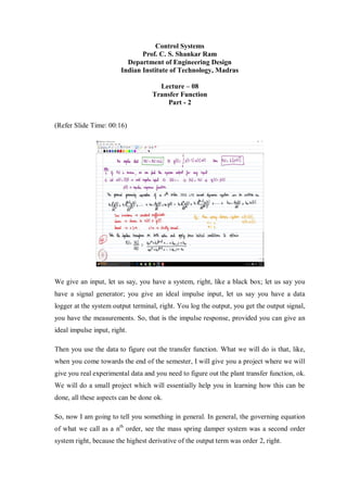
1. Control Systems
Prof. C. S. Shankar Ram
Department of Engineering Design
Indian Institute of Technology, Madras
Lecture – 08
Transfer Function
Part - 2
(Refer Slide Time: 00:16)
We give an input, let us say, you have a system, right, like a black box; let us say you
have a signal generator; you give an ideal impulse input, let us say you have a data
logger at the system output terminal, right. You log the output, you get the output signal,
you have the measurements. So, that is the impulse response, provided you can give an
ideal impulse input, right.
Then you use the data to figure out the transfer function. What we will do is that, like,
when you come towards the end of the semester, I will give you a project where we will
give you real experimental data and you need to figure out the plant transfer function, ok.
We will do a small project which will essentially help you in learning how this can be
done, all these aspects can be done ok.
So, now I am going to tell you something in general. In general, the governing equation
of what we call as a nth
order, see the mass spring damper system was a second order
system right, because the highest derivative of the output term was order 2, right.

2. So, in general the governing equation of an nth order SISO LTI causal system can be
written as the following.
𝑎0
𝑑 𝑛
𝑦(𝑡)
𝑑𝑡 𝑛
+ 𝑎1
𝑑 𝑛−1
𝑦(𝑡)
𝑑𝑡 𝑛−1
+ ⋯ + 𝑎 𝑛−1
𝑑𝑦( 𝑡)
𝑑𝑡
+ 𝑎 𝑛 𝑦( 𝑡)
= 𝑏0
𝑑 𝑚
𝑢(𝑡)
𝑑𝑡 𝑚
+ 𝑏1
𝑑 𝑚−1
𝑢(𝑡)
𝑑𝑡 𝑚−1
+ ⋯ + 𝑏 𝑚−1
𝑑𝑢( 𝑡)
𝑑𝑡
+ 𝑏 𝑚 𝑢( 𝑡)
So, this, this is how in general the governing equation for the class of systems that we are
going to study would come up, ok. So, please note that this class of systems is modeled
by using a linear ode with a constant coefficient. So, immediately you can see that it is
linear in y and u, ok. It has constant coefficients that is reflective of time invariance. So,
let me write down all the implications, because just by looking at the equation you
should be able to tell things about the system, right.
So, time invariance is reflected by the fact that we have constant coefficients in the
above equation. The fact that it is linear is because the above equation is linear in u(t)
and y(t) and the derivatives of these variables. Causality is reflected by the fact that n is
greater than or equal to m, ok. When n is greater than m some people will call it a strictly
causal. So, I am just introducing you to some terms which you may encounter, right. So,
essentially causality is reflected by the fact that n is greater than or equal to m, ok.
So, that is how causality is reflected in this particular equation, ok. So, this is an nth
order
system, where n is the order of the highest derivative of the output term, ok. So, as an
example, for the mass spring damper system, what were the values of n and m?
If you look at the mass spring damper system, the input was the force f(t) right, the
output was the displacement x(t) correct. So, what, what was the value of n.
Student: 2.
2, because we had 𝑥̈. What about m?
Student: 0.
0, because there was no derivative of the out, force term at all right. On the right hand
side we had just f(t) right. So, immediately you see that n is greater than m, so that was a
causal system, right. So, that is a representation of a causal system; that means, that

3. before you give a force, the mass is not going to get displaced, right. So, only the current
displacement is going to depend on past and current force that you are giving to the
system right. So, that is how the different aspects of LTI causality are reflected in the
governing equation.
Now, this is something I am going to leave it to you as a homework problem, because we
did it in detail for the mass spring damper system, this is just a general case, ok. So, take
the Laplace transform on both sides and apply zero initial conditions to obtain
𝑃( 𝑠) =
𝑌(𝑠)
𝑈(𝑠)
, the plant transfer function, which will turn out as
𝑃( 𝑠) =
𝑏0 𝑠 𝑚
+ 𝑏1 𝑠 𝑚−1
+ ⋯ + 𝑏 𝑚−1 𝑠 + 𝑏 𝑚
𝑎0 𝑠 𝑛 + 𝑎1 𝑠 𝑛−1 + ⋯ + 𝑎 𝑛−1 𝑠 + 𝑎 𝑛
So, this I leave it to you as homework, ok.
So, once again pretty straightforward, you just take the Laplace transform on both sides.
If you apply all initial conditions to be zero, when you take the Laplace transform of the
nth derivative the only term which will remain is 𝑠 𝑛
𝑌(𝑠). Similarly when you take the
Laplace transform the n-1 derivative of y, if you apply all the initial conditions to be zero
the term which you will be left with is 𝑠 𝑛−1
𝑌(𝑠).
So, that is what you will be left with. Same story in the right hand side right, if you take
the Laplace transform of the m th derivative of the input, you will have 𝑠 𝑚
𝑈(𝑠). plus a
bunch of terms having initial conditions of the input.
Even that you take as zero, so you will be just left with 𝑠 𝑚
𝑈(𝑠), so you cross multiply.
This is what you would get ok. So, that is the plant transfer function in this particular
case. So, that is what we have as the plant transfer function. So, immediately we will see,
what really is the consequence, right. So, let us look at it further. So, immediately one
can observe that, the plant transfer function is a ratio of two polynomials in s, right.

4. (Refer Slide Time: 09:30)
So, one could say that P of s is a ratio of two polynomials n(s) by d(s), right. So, n(s) is
the numerator polynomial of order m.
So, similarly d(s) is a denominator polynomial and that is of order n. So, we see that the
plant transfer function in general is going to be a ratio of two polynomials in s; a
numerator polynomial and a denominator polynomial. So, for when n is greater than or
equal to m for a causal system, we are going to have what is called as a proper transfer
function, ok.
Transfer function is said to be proper when the order of the denominator polynomial is
greater than or equal to the order of the numerator polynomial, ok. And in this case
anyway we are dealing with causal systems, you know that is going to be true, ok.
So, for the class of systems that we are going to deal with, we are going to get proper
transfer functions. So, when n is strictly greater than m, we add the term strictly ok. We
are going to get what are called, what is called as a strictly proper transfer function ok,
that is what is going to result when n is strictly greater than m, ok.
So, that is essentially the definition of what is called as a proper transfer function and a
strictly proper transfer function. So, now we see that 𝑃( 𝑠) =
𝑛(𝑠)
𝑑(𝑠)
, right. So, we see
immediately that, if I calculate the roots of n(s), that is solve 𝑏0 𝑠 𝑚
+ 𝑏1 𝑠 𝑚−1
+ ⋯ +
𝑏 𝑚−1 𝑠 + 𝑏 𝑚 , the roots are called as, what would you call the roots of n of s as? So if

5. you solve this equation the numerator polynomial equals zero and you get particular
values of s, at those values of s what will happen to the transfer function, it will become
zero right, because the numerator becomes zero. So, the roots of n(s) or what are called
as the zeros of the transfer function. I hope it is clear why they are called zeros right, that
transfer function vanishes right.
So, similarly the roots of the polynomial P(s) that is we solved 𝑎0 𝑠 𝑛
+ 𝑎1 𝑠 𝑛−1
+ ⋯ +
𝑎 𝑛−1 𝑠 + 𝑎 𝑛 = 0. So, wherever I have the denominator polynomial to be zero, you can
immediately see that the transfer function becomes singular, right. So, the transfer
function is a complex valued function in the variable s.
Now the point is that if I have a complex function f(s) and in the s domain at certain
points the function does not exist and its derivatives do not exist, those values of s are
called as singular points or poles right. We discussed it sometime before when we briefly
discuss complex variables. So, consequently the roots of d(s) are called as the poles of
the transfer function, ok.
Student: So, can we (Refer Time:15:04) y n equal to n greater than (Refer Time;15:07)
causality.
Causality ok so, let me give you a very simple example right. So, just to convey that
point ok, let us let us do it aside, right. So, the question was how one could say that n
greater than or equal to m implies causality. Let me go the other way ok, I will show you
how m greater than n will mean non causality ok, let us let us do that way ok.

6. (Refer Slide Time: 15:37)
So, let us take a very simple case where 𝑦( 𝑡) =
𝑑𝑢(𝑡)
𝑑𝑡
right. So, what are the values of n
and m here? n is going to be.
Student: 0.
0, m is going to be 1 all right. Do you agree? Ok. So, here n is less than m. So, we have
gone to the other side right. So, now, how is it anticipating, a non causal system is
anticipatory. Why? Because what does the derivative do.
See, suppose just to convey it graphically so that way we have a better idea right. So, let
us say I plot u(t) versus t right, I give some arbitrary input, but let us say I am at this
instant of time, this is my current instant of time t. So, what does my derivative give me?
It is a rate of change, graphically it will give me the slope right and the value of the
slope.
So, in a certain sense I will know what is going to come up in the future. So I am basing
my output as the derivative of the input signal which will tell me what is going to come
in the future. So, my system output is, at this instant of time, is influenced by what input
will come in the next instant. So, it tries to anticipate right and take action. So, you can
see that how its non causal, right.

7. If let us say we are at this point and if
𝑑𝑢
𝑑𝑡
is positive the output will increase, right. If I am
at this point where u(t) has reached what to say maxima, local maxima then the
derivative will be zero, so output will be zero right. So, in a certain sense it tries to
anticipate what is happening that is why it becomes non causal. So, now, I hope you have
an intuitive understanding of why this implies anticipation, right.
So, what I will do is that I am going to leave you with a few problems to do, right. And
then we will come back in the next class and essentially discuss further, right. So, let us
look at a few exercise problems, right. So, what I am going to do is that I am going to
essentially write down governing ordinary differential equations for a few simple LTI
systems right, and then you need to calculate the transfer function and get the unit step
response, ok.
So, that is the exercise I am going to give you ok, or let us make life simpler, let us say
we calculate the unit impulse response. So, you just need to take the inverse Laplace
transform of the transfer function that is all I want, right.
So, in each case determine the plant transfer function, its poles and zeroes and calculate
its unit impulse response. So, let me leave you with a few problems. Of course, the
moment I say transfer function, obviously we should assume all initial conditions to be
zero all right, ok.
1) 𝑦̈( 𝑡) + 5𝑦̇( 𝑡) + 6𝑦( 𝑡) = 𝑢(𝑡)
2) 𝑦̈( 𝑡) + 𝑦( 𝑡) = 𝑢(𝑡)
3) 𝑦̈( 𝑡) + 𝑦̇( 𝑡) − 2𝑦( 𝑡) = 𝑢(𝑡)
So, derive the transfer function, find the poles, zeroes and calculate the unit impulse
response ok, we would start from here in the next class.