control systems nptel lecture 47

1. Control Systems
Prof. C. S. Shankar Ram
Department of Engineering Design
Indian Institute of Technology, Madras
Lecture – 47
Frequency Response
Part-1
Ok. So good morning, let us get started right ok. So, yesterday if you recall, we were
looking at the state space representation right. So, we looked at how to rewrite a nth
order ODE as a set of n first order ODEs, and the state space representation had two
equations in general right what was called as a state equation, which is a first order
vector ODE that provided the time evolution of the state variables. And then we had
what is called as an output equation right, so that related the system output to the state
vector and the system input ok. So, those were the two equations in the state space
representation, and we essentially did an example, where we rewrote the mass spring
damper system governing equation in the state space form right.
(Refer Slide Time: 01:18)
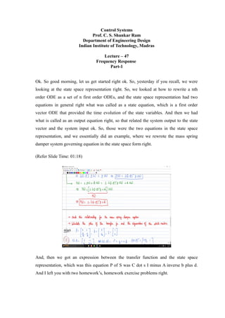
And, then we got an expression between the transfer function and the state space
representation, which was this equation P of S was C dot s I minus A inverse b plus d.
And I left you with two homework’s, homework exercise problems right.

2. (Refer Slide Time: 01:23)
So, I asked you to first check the relationship for the mass spring damper system and that
is what I just worked out here. So, this is the realization. So, the matrix A, the vector b
and vector c are these for the mass spring damper system. So, these are quantities which
you already derived yesterday. So, if you just work it out, calculate SI minus A and then
like SI minus A inverse, of course SI minus A inverse is going to be of course this
multiplied by 1 by determinant of SI minus A right, so that is the inverse ok, so that is
going to be SI minus A inverse and c dot SI minus A inverse b is going to be this. And if
you do the algebra, you will see that you will get the transfer function itself. So, just that
it is just an exercise to verify you know like our check the formula that we derived for
this particular example obviously, it must be true right.
And then like I asked you to calculate the poles of the transfer function and the eigen-
values of the state matrix. So, the poles of the transfer function are these ok. So, these are
the poles of the transfer function minus c plus or minus square root of c squared minus 4
mk divided by 2m. And we can see that the eigen-values of the state matrix also turn out
to be the same ok. So, in fact so to generalize of course, I am not telling the complete
picture, but then like by and large you know like for what are called as minimal
realizations ok. The poles of the transfer function and the eigenvalues of the state matrix
are the same ok.

3. (Refer Slide Time: 03:15)
Of course, this is true for what are called as minimal realization ok. So, we will see what
this is when we go to advanced courses on controls you know particularly on what is
called as modern control theory or state space theory ok. Yes, please.
Student: Sir, how was (Refer Time: 03:33).
How did you do that?
Student: (Refer Time: 03:36).
How did I do? What do you want, right.
Student: (Refer Time: 03:45).
Ok.
Student: (Refer Time: 03:51).
Ok. So first thing is that like you have SI minus A inverse to be a 2 by 2 matrix, first
multiply it by the vector b ok, which is a column vector 0 and 1 by m. So, if you multiply
that, you get this 1 by m and S by m right. And, then you have c, which is 1 0 you take
the dot product with that you will get 1 by m. See what is the dot product of 1 by 1 0 and
1 by m s by m? You will get 1 by m; 1 by m there is a m in the numerator you m and m

4. gets cancelled right. Look at 1 by m s squared plus c s plus k ok. So, this is the
determinant right.
See, what I have written here is the determinant right. So, the of course, this is the
reciprocal of the determinant this is 1 by determinant of SI minus A right. So, so what I
have done is that like determinant of SI minus A is s squared plus c by m s plus k m. This
can be rewritten as just s square plus sorry, m s square plus c s plus k divided by m all
right. So, I am just taking m as LCM. So, when you flip it, you will get m divided by m s
squared plus c s plus k and the m and 1 by m gets cancelled, so that is why you get 1 by
m s square plus c s plus k simple algebra ok.
Student: Sir.
Yeah.
Student: (Refer Time: 05:18).
So, that I am not touching upon here ok. So, essentially as I mentioned you know like
this concept of the set of poles or the plant transfer function being the same as eigen-
values of state matrix is true if the realization is minimal. So, what is a minimal
realization, I preemptively give you the answer, but then like you will understand it
better when you go to let us say modern control theory or an advanced course of control
that deals with state space. A minimal realization is one which is both completely
controllable and completely observable ok. So, then the question becomes you know
what is completely controllable and completely observable. So, you will see that that is
going to have a cascade effect, so we have to go deeper and deeper right.
So, essentially if you have a non-minimal realization by and large, you know like a the
one would be a subset of the other ok. This two sets will be exactly the same when you
have what is called as a minimal realization. So, here you see that there are two poles of
the transfer function and two eigen-values of the state matrix both are the same, so the
set is the same all right, so that is that is something which we can observe ok, yeah, fine.
So, but why is this important because you will immediately see that the what to say the
concept of stability right you in fact like we will learn what is called as stability about an
equilibrium state, when you go to state space based control. But, then you can

5. immediately feel that for a BIBO stability, we wanted all the poles to be the left of
complex plane right, if we use the transfer function approach.
So, similarly if I use the state space approach right for asymptotic stability what should I
have I should have all the eigen-values of the state matrix to be in the left half complex
plane, because the set is the same right. So, the task of ensuring asymptotic stability a
false boils down to the location of the poles of the transfer function or the eigen-values
of the state matrix ok, so that is that is that is the equivalence which I wanted to show
you here. Is it clear, what was the purpose behind this particular derivation right.
So, of course, we can go deeper and deeper, but I am not going to do that here because
our course is mainly focused on transfer function based analysis, but I just wanted to
give you an introduction to state space and we would learn more about this in advance
course of controls right ok.
(Refer Slide Time: 08:08)
So, let me now come back to our discussion using the transfer function ok. So, we are
going to discuss what is called as frequency response that is going to be something which
we are going to do for the next few classes, right. We are going to discuss what is called
as frequency response and how that is that can be used for control design ok, so that is
going to be the objective for this particular discussion right.

6. So, till now you know like if you recall what we have done right, predominantly we have
looked at the step response right. So, we have looked at the step response of dynamic
systems to essentially come up with performance parameters like definitions like time
constant, you know like rise time, settling time, peak overshoot and so on correct. So,
now we are going to analyze what happens when we provide a sinusoidal input to the
system and that is what frequency response deals with ok.
So, the term frequency response deals with the response of the system when a sinusoidal
I am sorry, input is provided to it ok, so that is what we are going to look at. By and large
we are going to look at what to say the steady state response ok, we will say why ok. So,
what we will first consider is that like let us consider a stable this is very important of
course, we can only talk about performance only if we have a stable system to begin with
right there is something which we already discussed right.
So, let us consider a stable LTI causal SISO dynamic system whose transfer function is P
of S ok. So, let us say we consider a plant or a system with a transfer function P of S. So,
what do we have, so we have the system transfer function to be P of S, so we provide an
input U whose Laplace transform is U of s and we get an output Y, so whose Laplace
transform is Y of s right. So, immediately we know that Y of s is going to be equal to P
of s times U of s ok.
So, let us consider u of t to be sum U naught sin omega t ok, so that is like we are
considering a sinusoidal input, so where u of t is sum U naught sin omega t ok. So, the
input has a frequency omega and a magnitude of U naught right. And consequently what
is going to happen to the Laplace transform so we are going to get U of s to be equal to U
naught omega divided by s squared plus omega squared ok. So, that is what we are going
to have right, if I take the Laplace transform of this particular signal U naught is the
magnitude all right, so that is a constant positive real number right. So, on the frequency
of the input is omega so that is what we are going to have for U of s right.
And, so let us say P of s be sum n of s divided by d of s so this I can rewrite as n of s
divided by let us say s plus p 1, s plus p 2, s plus p n ok. But, and what do we know
about all the poles of P of s?
Student: (Refer Time: 12:34)

7. All poles of a P of s lie in the left of complex plane right. Why, because we are assuming
a stable system to begin with right. So, all poles of P of s lie in the LHP right, so that is
something which we already have presumed right in this particular discussion ok.
(Refer Slide Time: 13:06)
So, let us now you know like process this particular equation. So, this implies a Y of s is
equal to P of s times U of s that is going to be equal to sum n of s divide d by d of s times
U naught omega divided by s square plus omega square correct, so that is something
which we. So, this I can rewrite the as sum a 1 divided by s plus j omega plus a 2 divided
by s minus j omega plus sum n 1 of s divided by d of s ok. So, I am just start doing
partial fraction expansion right.
See, because what has happened like so the plant transfer function is n of s divided by d
of s then I multiply it with a second order term denominator is s squared plus omega
square. So, what I am doing is that I am writing s squared plus omega squared as s plus j
omega times s minus j omega I can do that right.
So, essentially then we are doing partial fraction expansion. So, I will write for s plus j
omega a 1 b y s plus j omega and then s minus j omega the residue I take it as a 2, so I
get a 2 by s minus j omega plus sum n 1 of s. You know whatever is left behind divided
by d of s d of s is the original denominator polynomial s plus p 1 all the way till s plus p
n ok, so that is my output right, so and that is essentially this ok. So, this is nothing but
please note then this is P of s ok, please remember that ok.

8. So, if I want to find a 1 and a 2, what should I do now? Let us say I want to find a 1,
what should we do, we multiply both sides by s plus j omega right. So, if I do this, what
will I get, I will get P of s U naught omega divided by s minus j omega that is what will
happen to the left hand side. On the right hand side, I will get a 1 a 2 times s plus j
omega divided by s minus j omega plus sum n 1 of s which is left behind right times s
plus j omega divided by d of s right. So, this is what I will get right, if I multiply both
sides by this one.
So, now what should I do, I should substitute the root right of that factor which is s
equals minus j omega, I can do this. So, then what will I get, I will get P of minus j
omega U naught omega divided by what will happen to the denominator it will be minus
j omega minus j omega I will get minus 2 j omega and that is going to be equal to a 1
right ok. So, this implies that the residue a 1 is going to be equal to U naught divided by
2 j right, omega and omega cancelled now times P of minus j omega ok.
So, what is P of minus j omega P of minus j omega is the plant transfer function
evaluated at s equals minus j omega, obviously that is going to be a complex quantity
right. So, and we know that any complex variable has a magnitude and a phase right. So,
then there are various representations of a complex variable right. I can have a
representation in terms of real and complex part, I can have a magnitude and a phase
representation also for the same complex variable right.
So, now what we do then, if I have a complex variable P of j omega, I can rewrite this as
the magnitude of P of j omega times e power j phi, where phi is the phase of P of j omega
right. This is one representation of a complex variable. Do you agree? Yeah.
Student: (Refer Time: 17:38) a 1 minus (Refer Time: 17:39).
Yes, I missed it minus thank you, you are right, thank you ok, so yeah, so that is minus u
naught by 2 j p of minus j omega right. So, I get this right. So, this immediately implies
that if I have P of minus j omega what am I going to have that is going to be P of j omega
e power minus j phi ok, so the phase just becomes negative of P of j omega all right, so
that is the representation which we are going to follow all right for the complex valued
function p of j omega ok.

9. So, once I have this what is going to happen to a 1 this implies in a 1 is going to be
minus U naught divided by 2 j the magnitude of P of j omega e power j phi ok. Please
remember what is phi, phi is the phase of P of j omega, obviously phi depends on omega
right you vary the frequency obviously the phase also varies right so that is what we have
for a 1 ok.
(Refer Slide Time: 19:02)
Now, similarly let us figure out a 2 right. So, let us get the expression for a 2. So, if I
want the expression for a 2, what do I do, I multiply both sides by s minus j omega all
right. So, this implies that I will get P of s U naught omega divided by s plus j omega that
is going to be equal to a 1 plus a 2 sorry a 1 s plus sorry what is going to happen I
multiplied by s minus j omega right. So, I will have a 1 s minus j omega divided by s
plus j omega plus a 2 plus n 1 of s minus j omega divided by d of s all right so that is
what I will have correct. I hope everyone agrees.
Now, what should I do, here I substitute s equals j omega right that is the root of this
particular factor. So, what will I immediately get, I will get P of j omega U naught omega
divided by 2 j omega that is going to be equal to a 2 all right. So, omega and omega will
immediately cancels. So, a 2 is going to be u naught by 2 j P of j omega then I just
represent P of j omega as the magnitude of P of j omega e power j phi right. So, we are
almost done ok. So, we are almost there just a few more steps ok.

10. Now, let us go back here right. So, our Y of s is going to be a 1 divided by s plus j omega
plus a 2 divided by s minus j omega plus n 1 by d of s right. So, let me write it down. So,
our Y of s is going to be a 1 divided by s plus j omega plus a 2 divided by s minus j
omega plus n 1 of s divided by sum d of s this immediately implies there. If I take the
inverse Laplace transform, what will I get, what will be the inverse Laplace transform of
the first term I will get e a 1 e power minus j omega t right correct. And then I will get
for the second term a 2 e power j omega t right.
And what is going to happen to the next term you know like so essentially let there be k
distinct poles, this is something which we already done right for a nth order system. Let
us say let there be k distinct poles. The inverse Laplace transform of this term is going to
be the following right, so this is something which we have already done, so please go
back and look at that. So, let us say let there be k distinct poles with mu I being the
multiplicity of each pole we have already figure out what is the inverse Laplace
transform right so this is what we will have all right.
So, the main thing is that like we are going to have the poles as the exponents right. So,
this is something if you recall which we did when we analyze stability, if you recall. And
this is the result where we use to figure out that if my poles lie in the left of complex
plane, the system is going to be BIBO stable right. So, if you recall that is what we did
sometimes some classes back. So, essentially I am just going to get the same structure
right, so that is very important as far as this is concerned.