Download as PDF, PPTX


![Active Shape Model (T. Cootes et al., 1995)
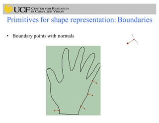
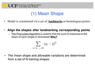
• Representation of Shapes
– Point Distribution Model (PDM)
– Represent a shape instance by a judiciously chosen set of points
(features), each of which is a k-dim vector. N feature points are
stacked into a long vector of length kn:
where
23
q = [p1, . . . , pn]T
pi = (xi, yi), for i = 1, ..., n
landmarks](https://image.slidesharecdn.com/lec12-170330052350/85/Lec12-Shape-Models-and-Medical-Image-Segmentation-23-320.jpg)
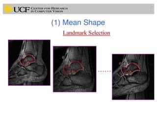
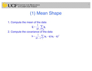
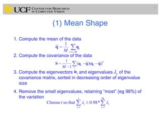
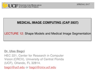
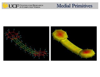
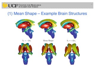
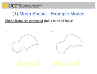
![(1) Mean Shape – Model Variation
• We now approximate any instance of the shape, including
the training instances, by projecting onto the first t
eigenvectors:
• The weight vector b is identified as the characteristic of this
instance of the shape:
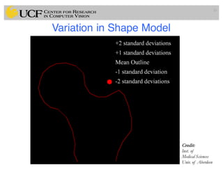
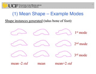
• Varying the weights bi enables us to explore the allowable
variations in the shape!
32
q = ¯q +
tX
i=1
biui
b = [b1, ..., bt]T](https://image.slidesharecdn.com/lec12-170330052350/85/Lec12-Shape-Models-and-Medical-Image-Segmentation-32-320.jpg)
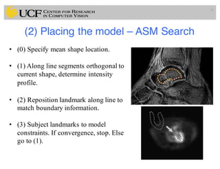
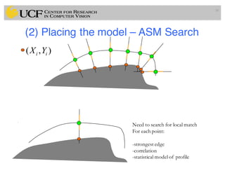
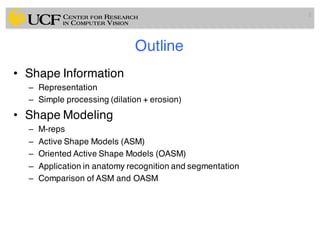
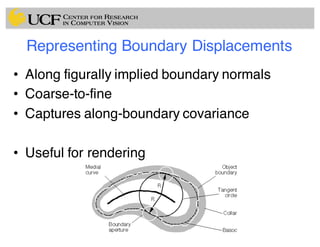
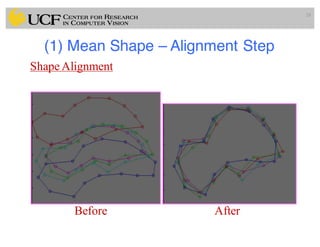
![Finding the model pose & parameters
• Suppose we have identified a set of points Y in the image.
Evidently, we can seek to minimize the squared distance:
Algorithm
1. Initialize b=0
2. Generate initial model instance
3. Find T that best aligns q to Y (e.g., similarity transform)
4. Invert pose parameters, to project into model frame
5. Update the model parameters:
6. Repeat from step 2 until convergence
40
|Y T(¯q +
tX
i=1
biui)|2
q = (¯q +
tX
i=1
biui)
y = T 1
(Y)
b = UT
(y ¯q) U = [u1|u1|...ut]](https://image.slidesharecdn.com/lec12-170330052350/85/Lec12-Shape-Models-and-Medical-Image-Segmentation-40-320.jpg)
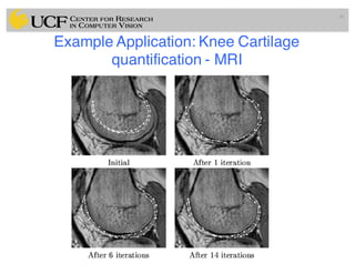
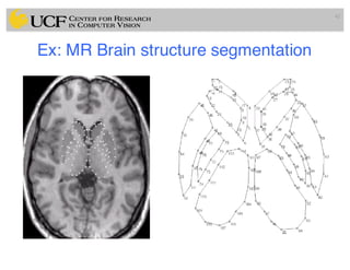
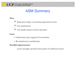
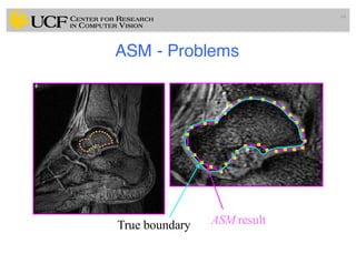
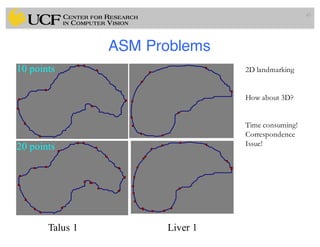
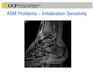
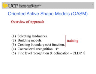
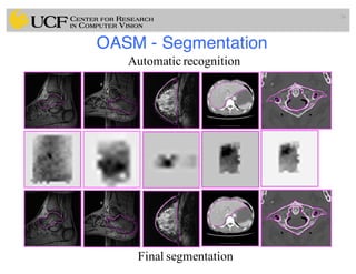
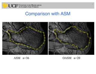
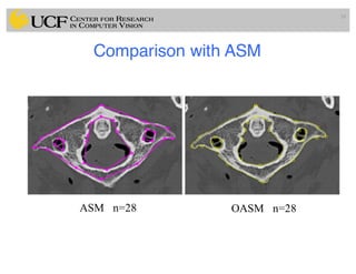
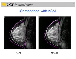
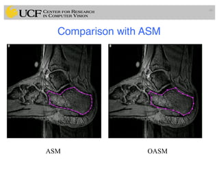
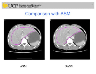
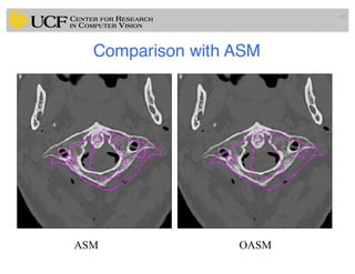
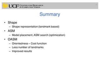

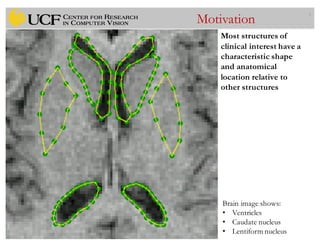
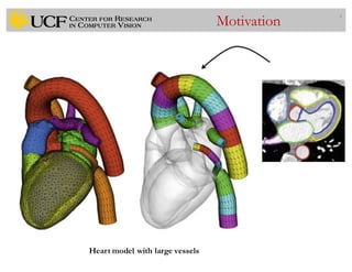
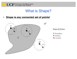
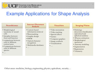
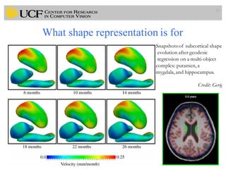
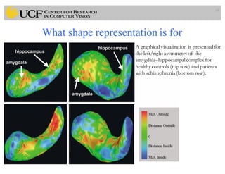
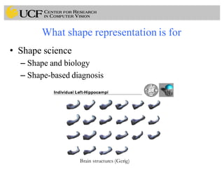
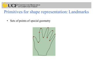
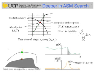
This document outlines a lecture on shape models and medical image segmentation, addressing the importance of shape in medical imaging and various shape modeling techniques such as active shape models (ASM) and oriented active shape models (OASM). It details the applications of shape analysis in fields like neuroscience, visual arts, and imaging, while also discussing the methodologies for model construction, landmark selection, and optimization in image segmentation. Additionally, comparisons between ASM and OASM highlight improvements in segmentation accuracy and efficiency.