Download as PDF, PPTX


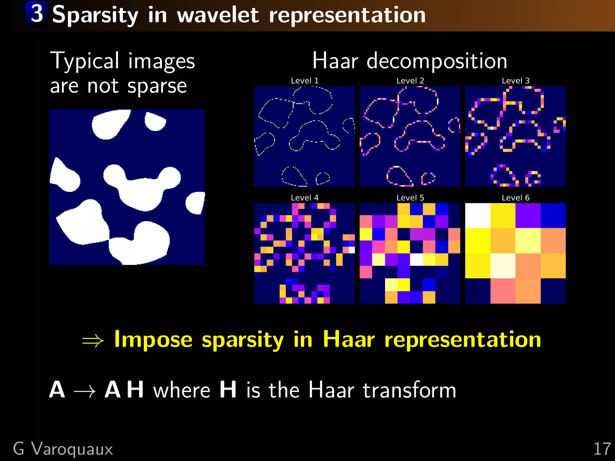
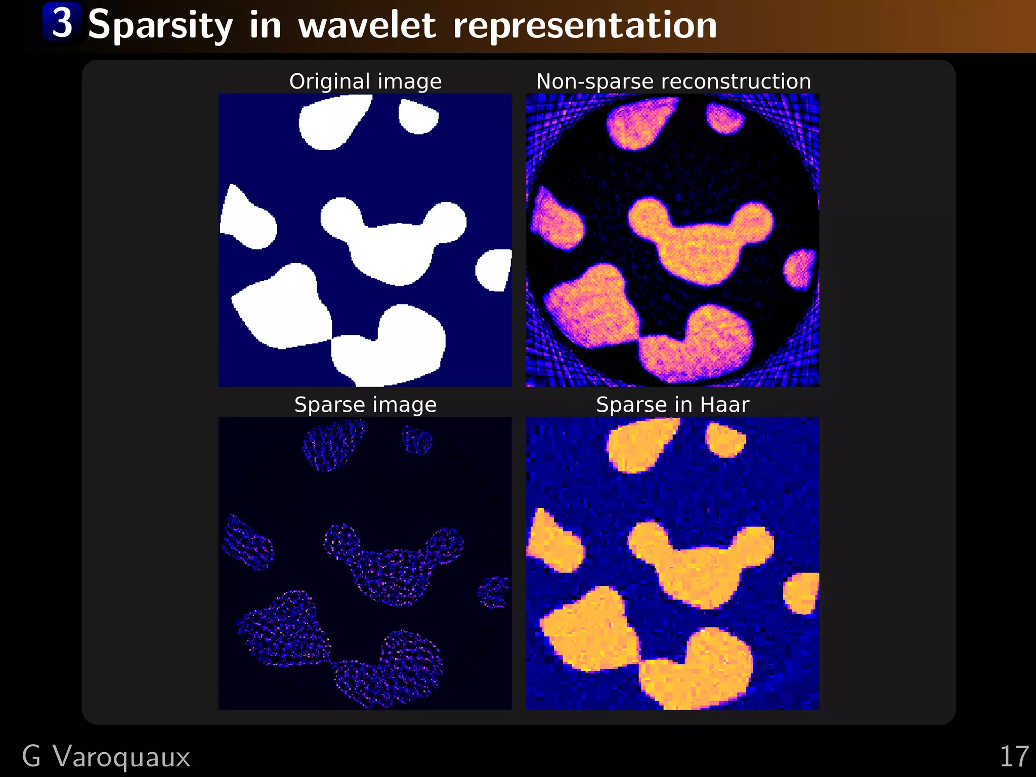
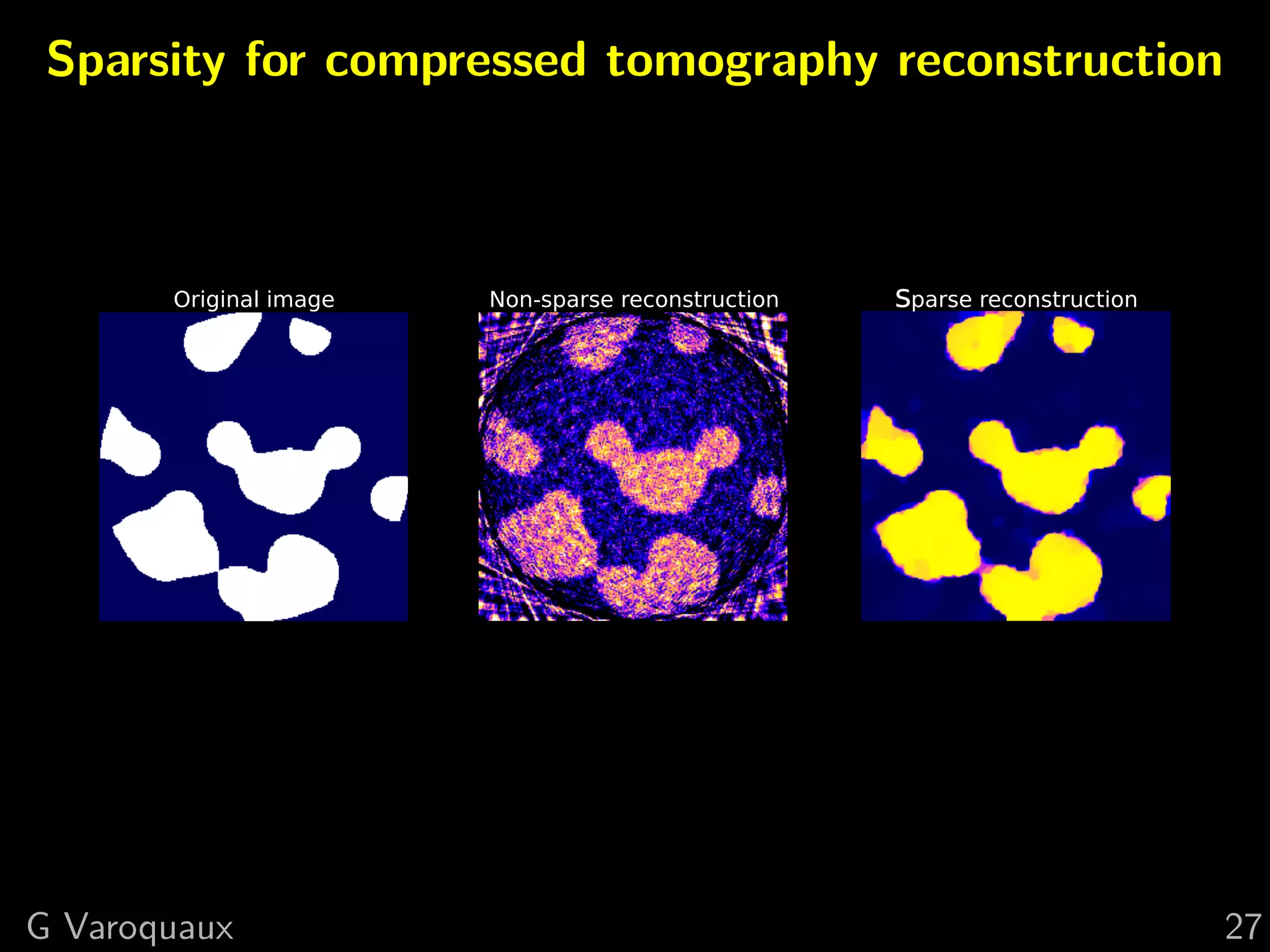
![Recovery of sparse signal
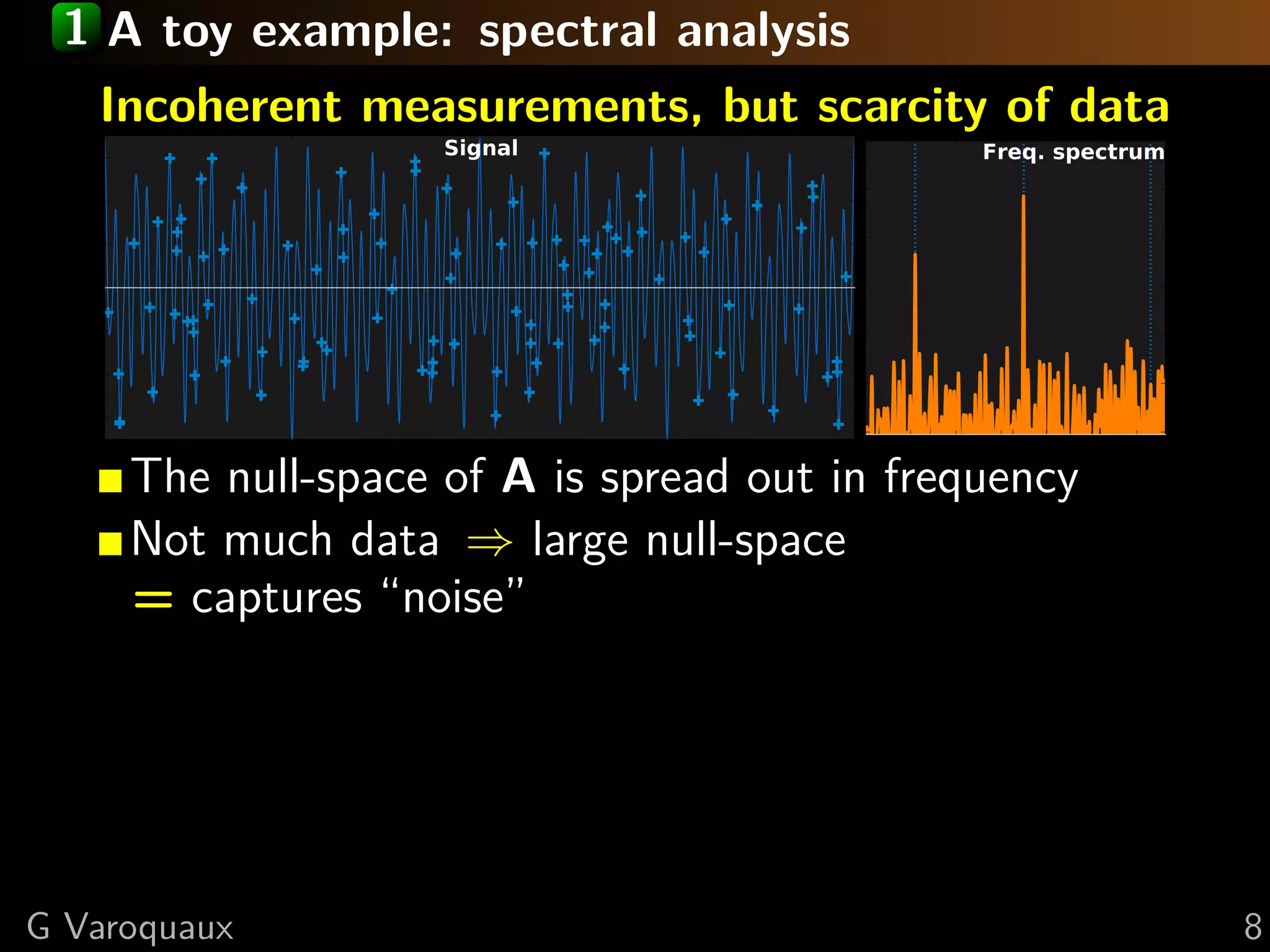
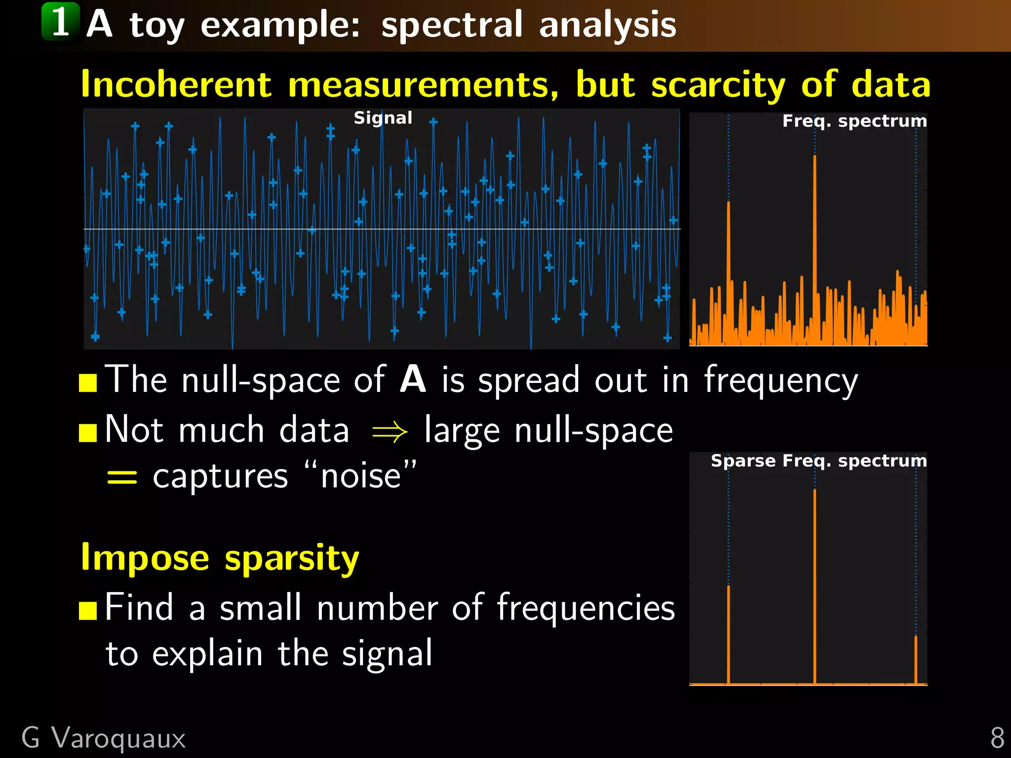
Null space of sensing operator incoherent
with sparse representation
⇒ Excellent sparse recovery with little projections
Minimum number of observations necessary:
nmin ∼ k log p, with k: number of non zeros
[Candes 2006]
Rmk Theory for i.i.d. samples
Related to “compressive sensing”
G Varoquaux 11](https://image.slidesharecdn.com/slides-121210235817-phpapp01/75/A-hand-waving-introduction-to-sparsity-for-compressed-tomography-reconstruction-17-2048.jpg)
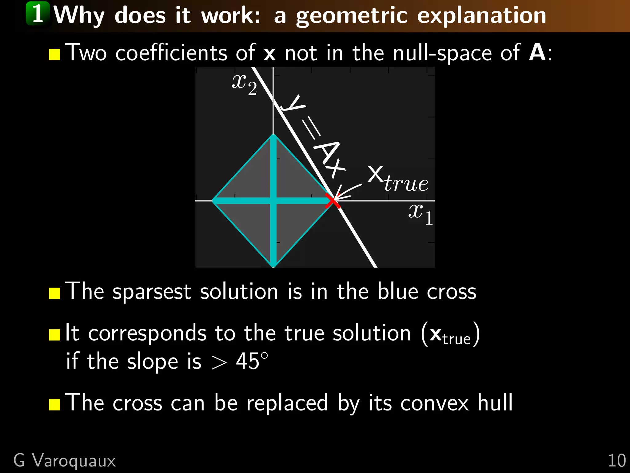
![2 Maximizing the sparsity
0 number of non-zeros
min 0(x)
x
s.t. y = A x
x2
y=
Ax
xtrue
x1
“Matching pursuit” problem [Mallat, Zhang 1993]
“Orthogonal matching pursuit” [Pati, et al 1993]
Problem: Non-convex optimization
G Varoquaux 13](https://image.slidesharecdn.com/slides-121210235817-phpapp01/75/A-hand-waving-introduction-to-sparsity-for-compressed-tomography-reconstruction-19-2048.jpg)
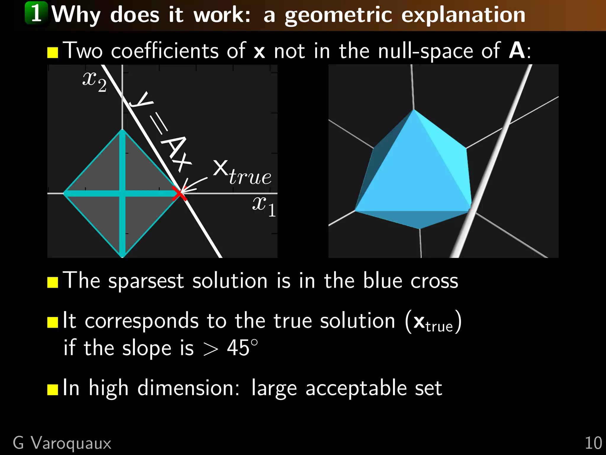
![2 Maximizing the sparsity
1 (x) = i |xi |
min 1(x)
x
s.t. y = A x
x2
y=
Ax
xtrue
x1
“Basis pursuit” [Chen, Donoho, Saunders 1998]
G Varoquaux 13](https://image.slidesharecdn.com/slides-121210235817-phpapp01/75/A-hand-waving-introduction-to-sparsity-for-compressed-tomography-reconstruction-20-2048.jpg)
![2 Modeling observation noise
y = Ax + e e = observation noise
New formulation:
2
min 1 (x)
x
s.t. y = A x y − Ax 2 ≤ ε2
Equivalent: “Lasso estimator” [Tibshirani 1996]
2
min y − Ax
x 2 + λ 1(x)
G Varoquaux 14](https://image.slidesharecdn.com/slides-121210235817-phpapp01/75/A-hand-waving-introduction-to-sparsity-for-compressed-tomography-reconstruction-21-2048.jpg)
![2 Modeling observation noise
y = Ax + e e = observation noise
New formulation:
2
min 1 (x)
x
s.t. y = A x y − Ax 2 ≤ ε2
Equivalent: “Lasso estimator” [Tibshirani 1996]
2
x2
min y − Ax
x 2 + λ 1(x)
Data fit Penalization x1
Rmk: kink in the 1 ball creates sparsity
G Varoquaux 14](https://image.slidesharecdn.com/slides-121210235817-phpapp01/75/A-hand-waving-introduction-to-sparsity-for-compressed-tomography-reconstruction-22-2048.jpg)
![2 Probabilistic modeling: Bayesian interpretation
P(x|y) ∝ P(y|x) P(x) ( )
“Posterior” Forward model “Prior”
Quantity of interest Expectations on x
Forward model: y = A x + e, e: Gaussian noise
⇒ P(y|x) ∝ exp − 2 1 2 y − A x 2
σ 2
1
Prior: Laplacian P(x) ∝ exp − µ x 1
1 2 1
Negated log of ( ): 2σ 2 y − Ax 2 + µ 1 (x)
Maximum of posterior is Lasso estimate
Note that this picture is limited and the Lasso is not a good
G Varoquaux Bayesian estimator for the Laplace prior [Gribonval 2011]. 15](https://image.slidesharecdn.com/slides-121210235817-phpapp01/75/A-hand-waving-introduction-to-sparsity-for-compressed-tomography-reconstruction-23-2048.jpg)
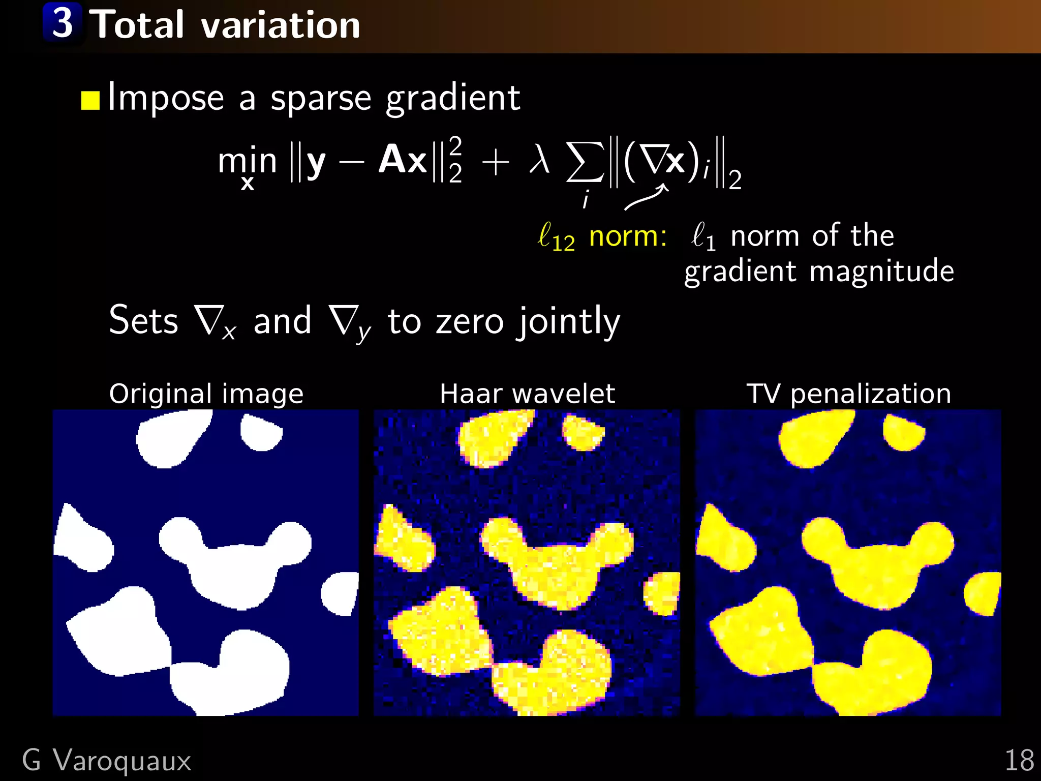
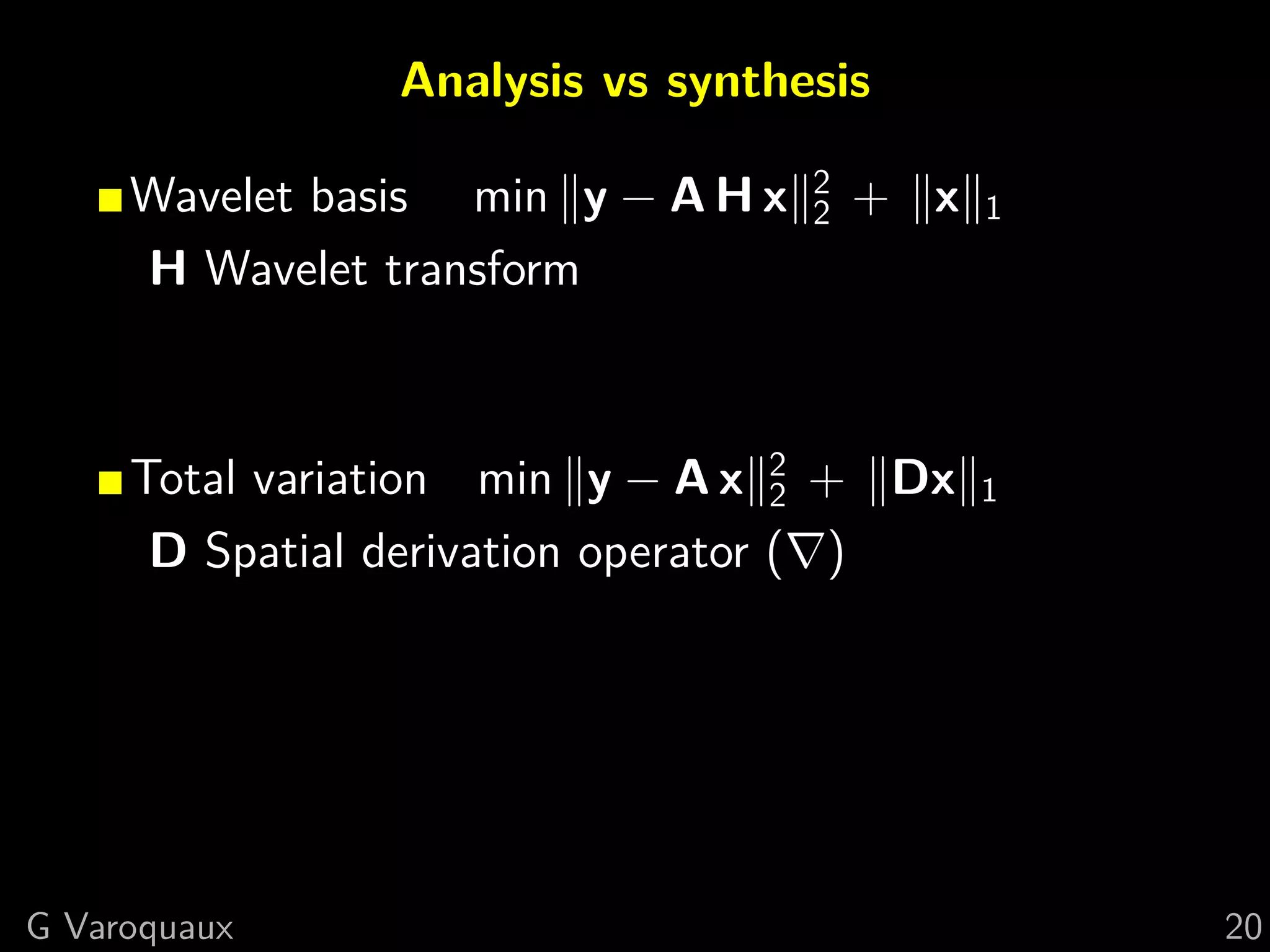
![3 Total variation + interval
Bound x in [0, 1]
2
min y−Ax
x 2+λ ( x)i 2 +I([0, 1])
i
Original image TV penalization TV + interval
G Varoquaux 19](https://image.slidesharecdn.com/slides-121210235817-phpapp01/75/A-hand-waving-introduction-to-sparsity-for-compressed-tomography-reconstruction-29-2048.jpg)
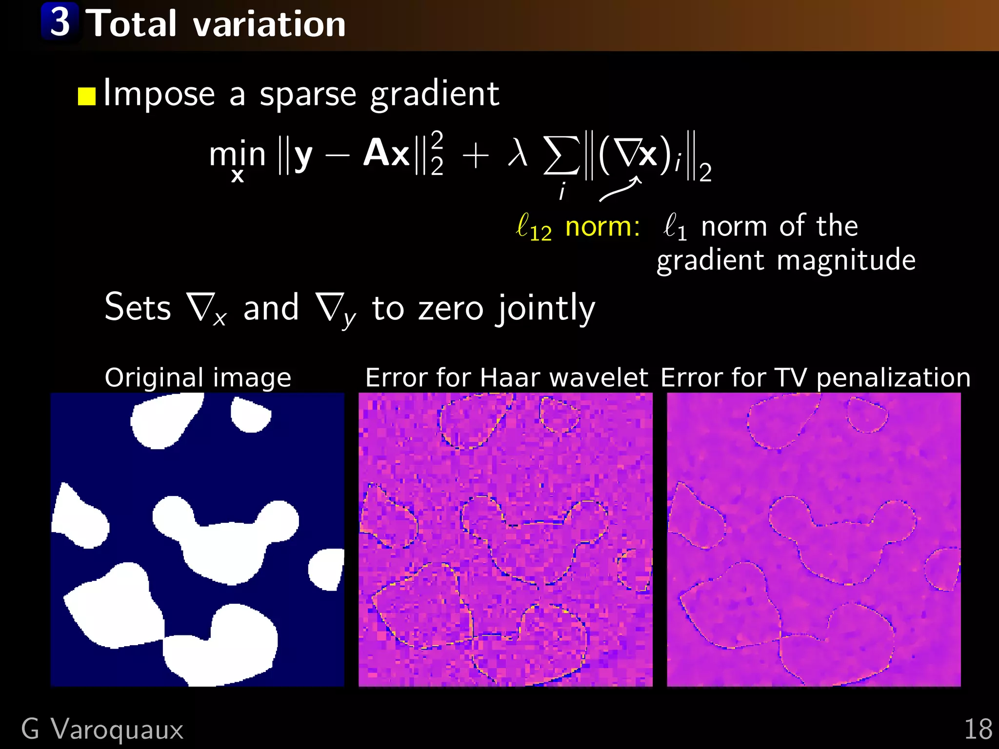
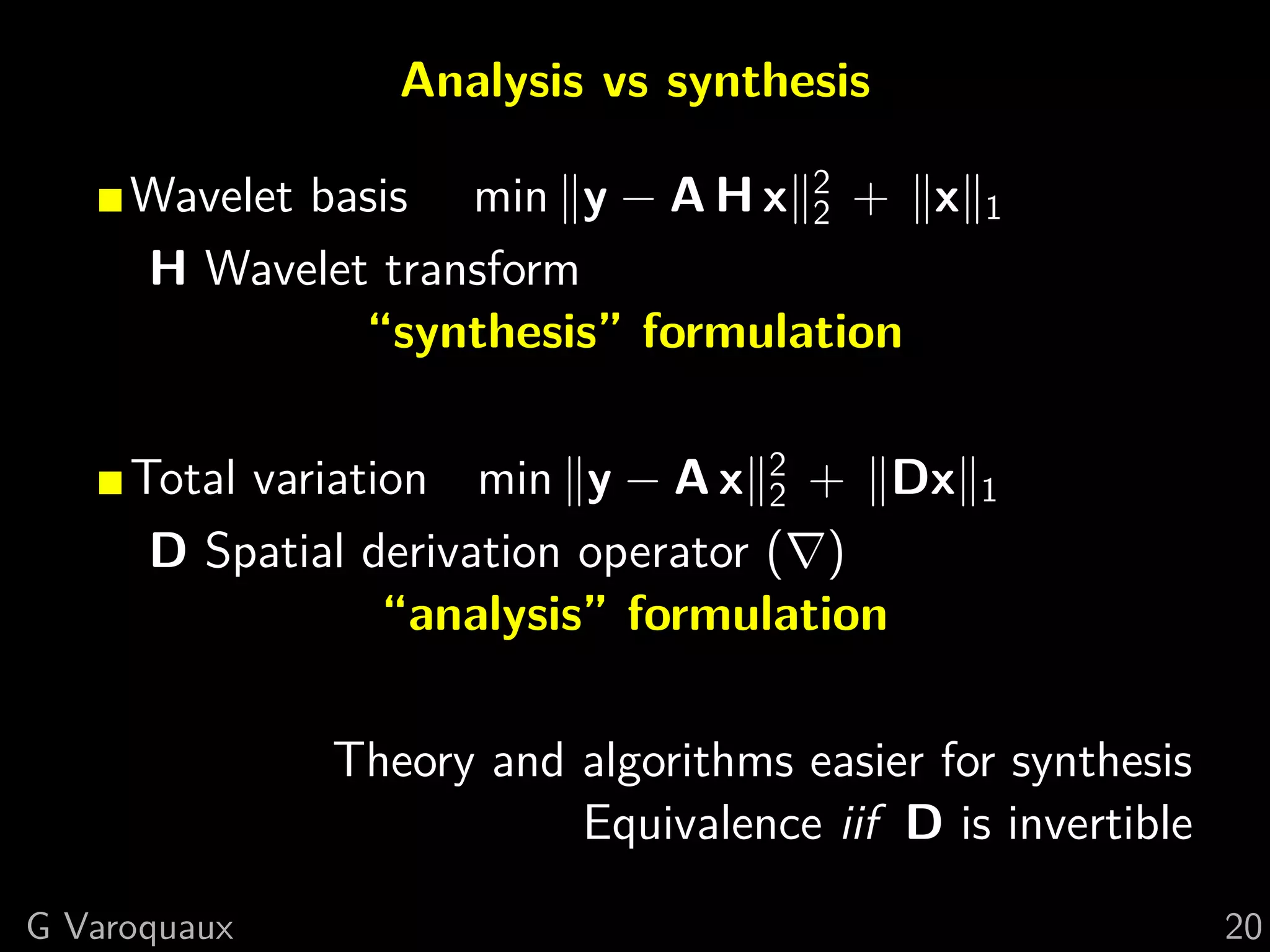
![3 Total variation + interval
Bound x in [0, 1]
2
min y−Ax
x 2+λ ( x)i 2 +I([0, 1])
i
TV Rmk: Constraint
Histograms: TV + interval does more than fold-
ing values outside of
the range back in.
0.0 0.5 1.0
Original image TV penalization TV + interval
G Varoquaux 19](https://image.slidesharecdn.com/slides-121210235817-phpapp01/75/A-hand-waving-introduction-to-sparsity-for-compressed-tomography-reconstruction-30-2048.jpg)
![3 Total variation + interval
Bound x in [0, 1]
2
min y−Ax
x 2+λ ( x)i 2 +I([0, 1])
i
TV Rmk: Constraint
Histograms: TV + interval does more than fold-
ing values outside of
the range back in.
0.0 0.5 1.0
Original image Error for TV penalization Error for TV + interval
G Varoquaux 19](https://image.slidesharecdn.com/slides-121210235817-phpapp01/75/A-hand-waving-introduction-to-sparsity-for-compressed-tomography-reconstruction-31-2048.jpg)
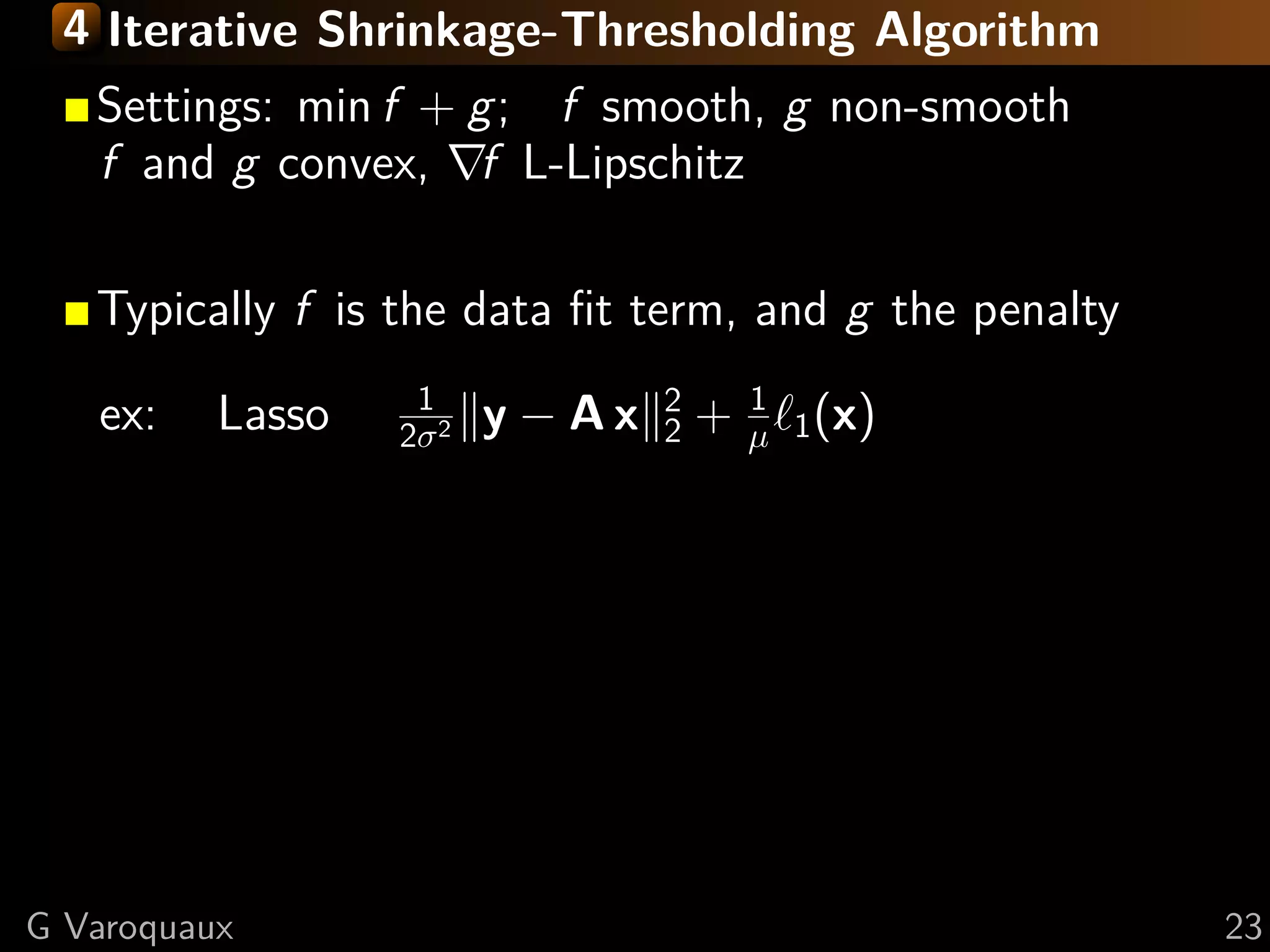
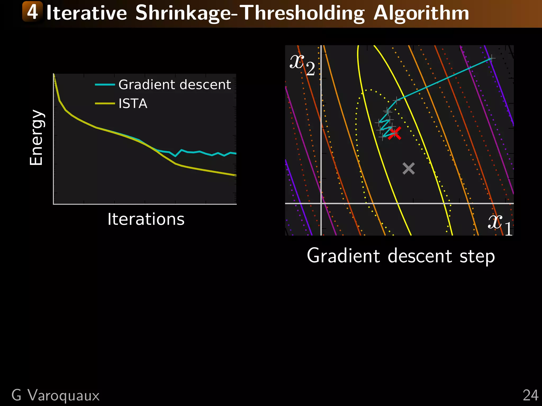
![4 Iterative Shrinkage-Thresholding Algorithm
Settings: min f + g; f smooth, g non-smooth
f and g convex, f L-Lipschitz
Minimize successively:
(quadratic approx of f ) + g
f (x) < f (y) + x − y, f (y)
2
+L x − y
2 2
Proof: by convexity f (y) ≤ f (x) + f (y) (y − x)
in the second term: f (y) → f (x) + ( f (y) − f (x))
upper bound last term with Lipschitz continuity of f
L 1 2
xk+1 = argmin g(x) + x − xk − f (xk ) 2
x 2 L
[Daubechies 2004]
G Varoquaux 23](https://image.slidesharecdn.com/slides-121210235817-phpapp01/75/A-hand-waving-introduction-to-sparsity-for-compressed-tomography-reconstruction-37-2048.jpg)
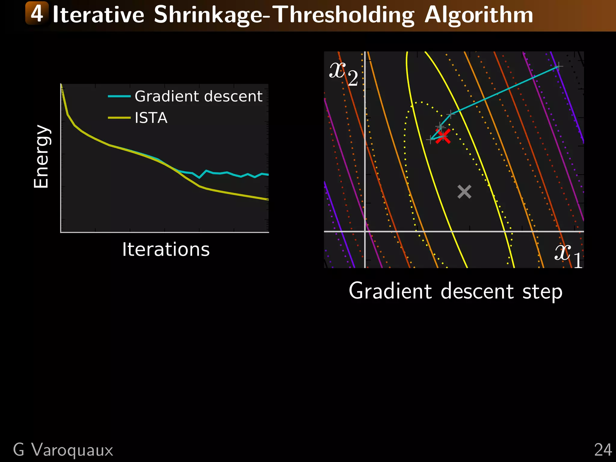
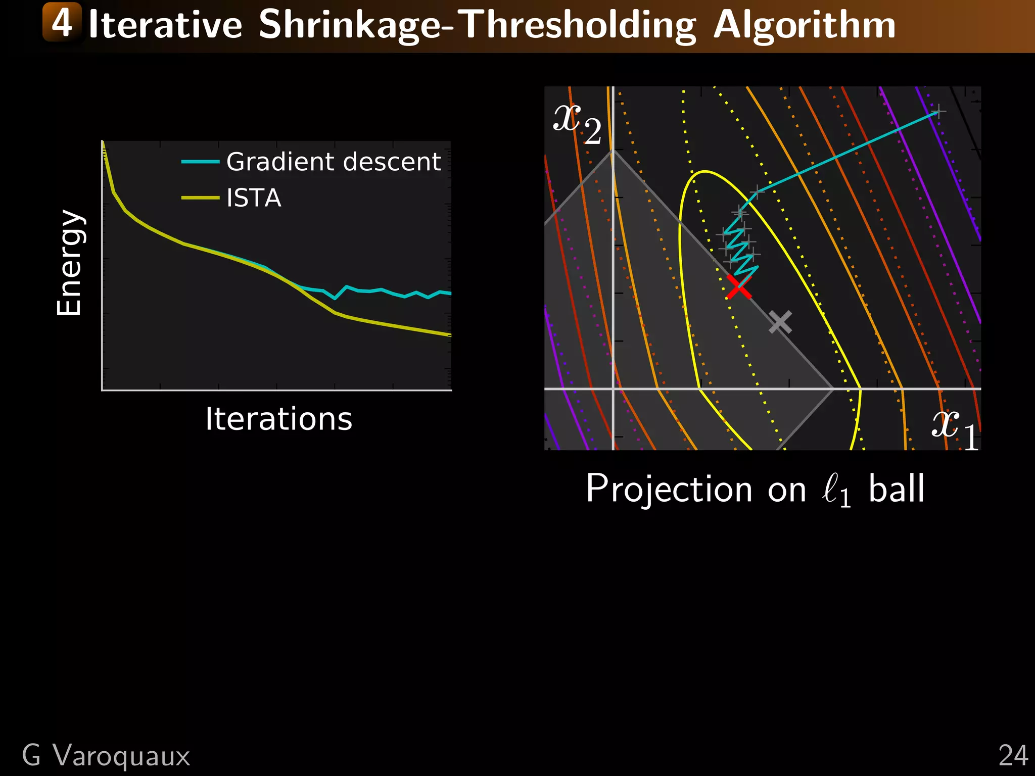
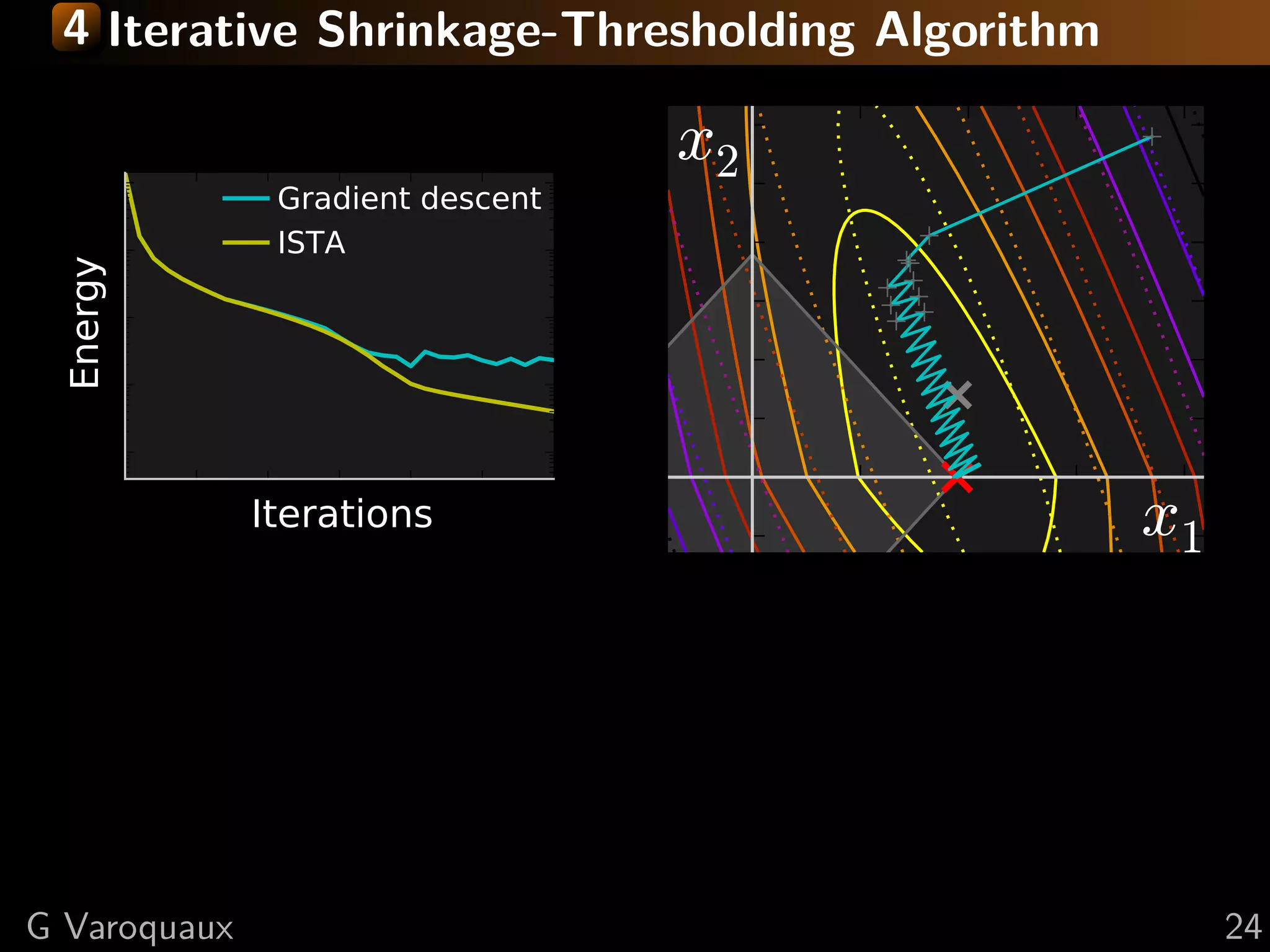
![4 Iterative Shrinkage-Thresholding Algorithm
Step 1: Gradient descentsmooth, g non-smooth
Settings: min f + g; f on f
f and g convex, f L-Lipschitz
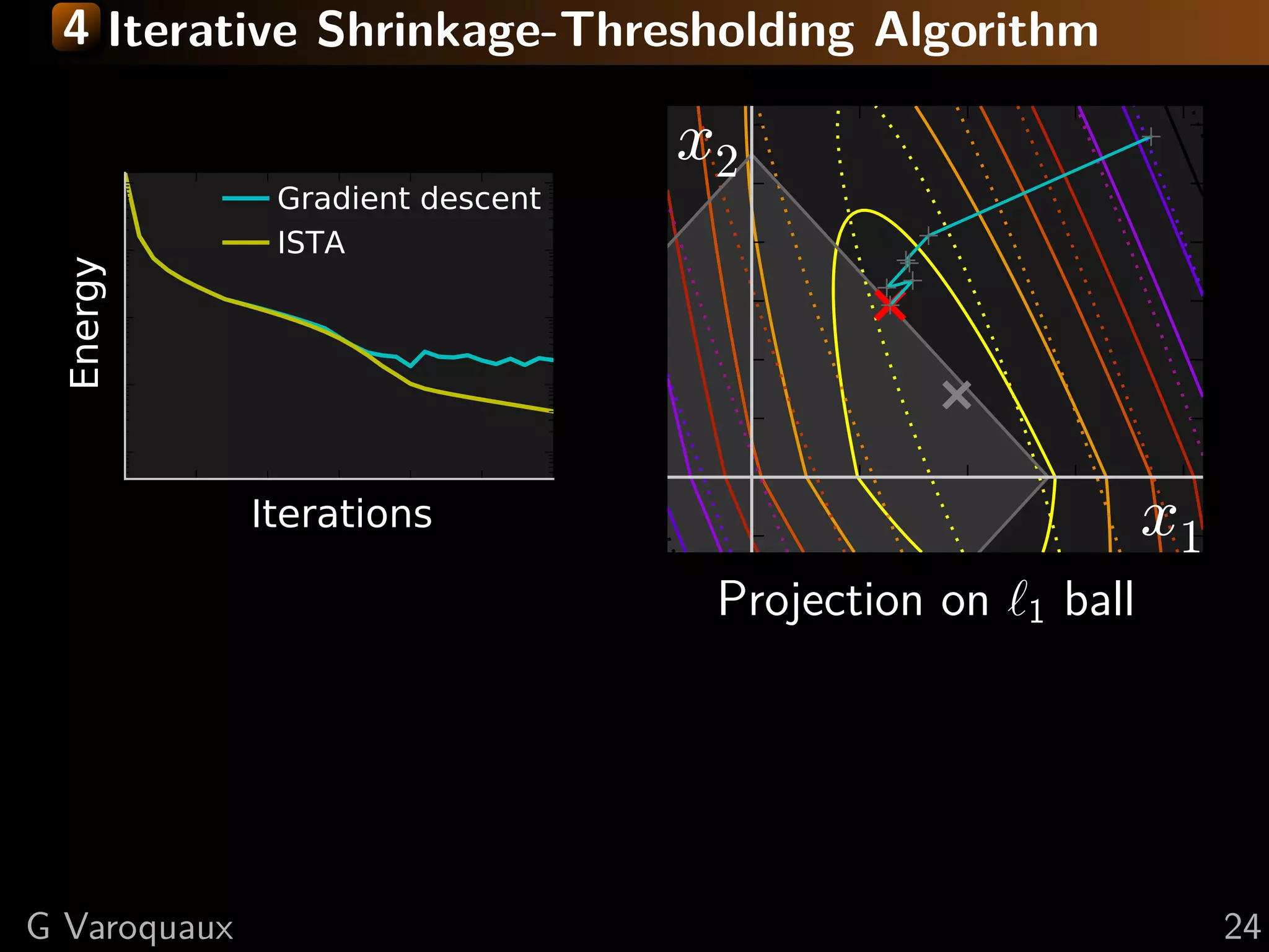
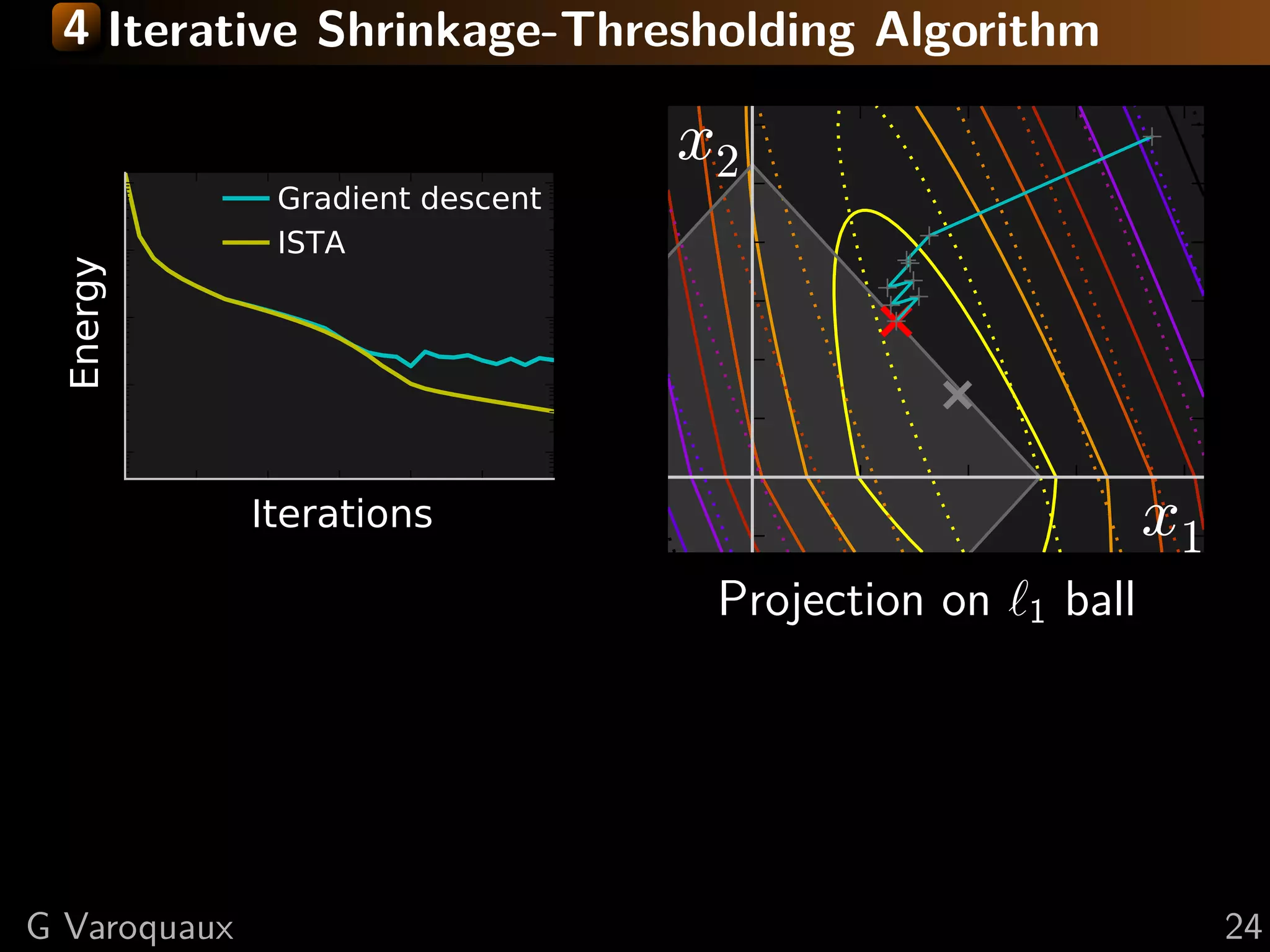
Step 2: Proximal operator of g:
Minimize proxλg (x) def argmin y − x 2 + λ g(y)
successively:
= 2
y
(quadratic approx of f ) + g
Generalization of Euclidean projection
f (x) < f (y) + x − y, f (y)1}
on convex set {x, g(x) ≤ 2 Rmk: if g is the indicator function
+L x − y 2
2
of a set S, the proximal operator
is the Euclidean projection.
Proof: by convexity f (y) ≤ f (x) + f (y) (y − x)
prox
in theλ
1
(x) = sign(x ) x − λ
second term: f (y) → f (x) + ( i f (y) − f (x))
i +
upper bound last term with Lipschitz continuity of f
“soft thresholding”
L 1 2
xk+1 = argmin g(x) + x − xk − f (xk ) 2
x 2 L
[Daubechies 2004]
G Varoquaux 23](https://image.slidesharecdn.com/slides-121210235817-phpapp01/75/A-hand-waving-introduction-to-sparsity-for-compressed-tomography-reconstruction-38-2048.jpg)


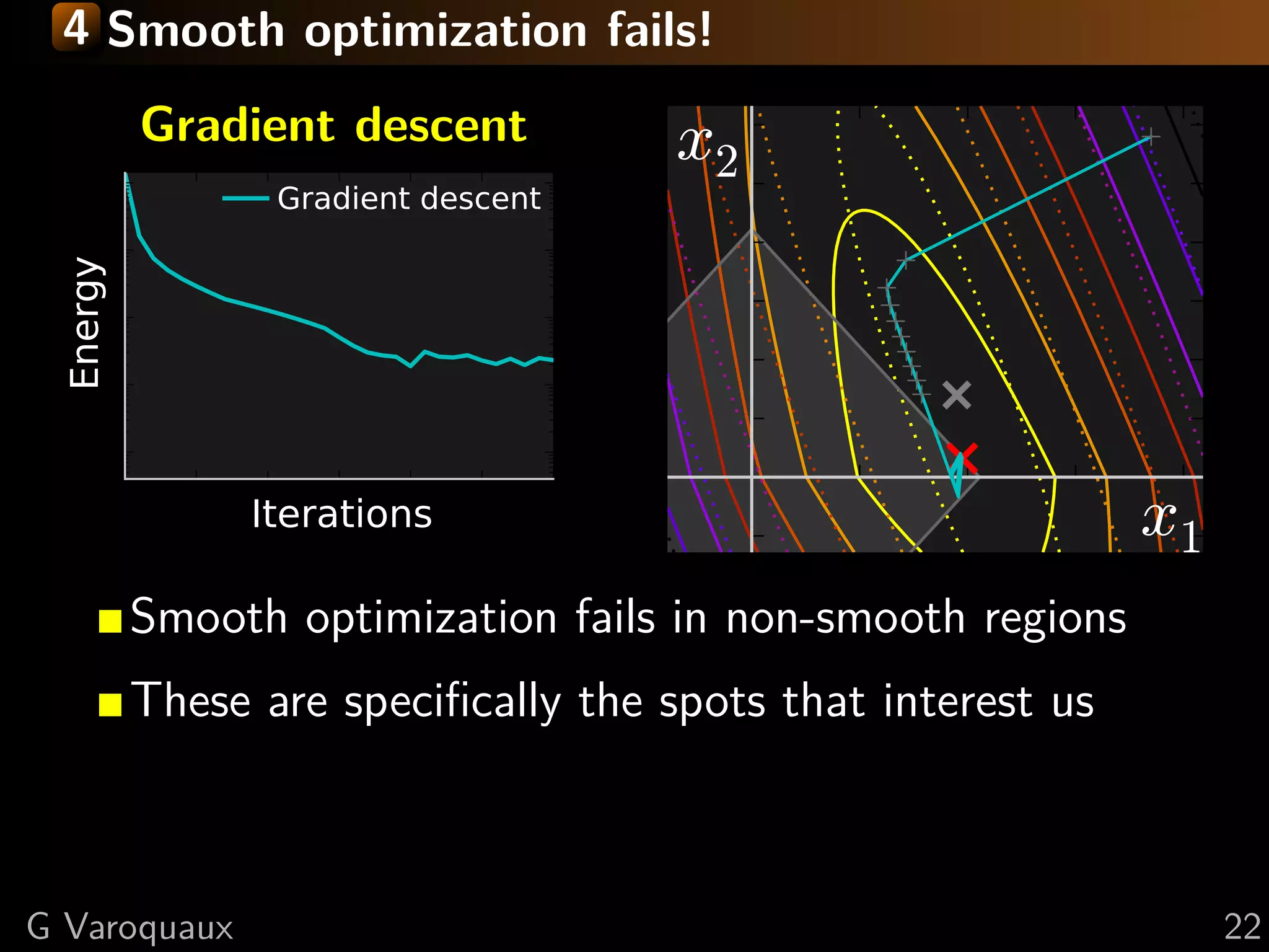
![4 Fast Iterative Shrinkage-Thresholding Algorithm
FISTA
Gradient descent
x2
ISTA
FISTA
Energy
Iterations x1
As with conjugate gradient: add a memory term
ISTA tk −1
dxk+1 = dxk+1 + tk+1 (dxk − dxk−1 ) √
1+ 2
1+4 tk
t1 = 1, tk+1 = 2
⇒ O(k −2 ) convergence [Beck Teboulle 2009]
G Varoquaux 25](https://image.slidesharecdn.com/slides-121210235817-phpapp01/75/A-hand-waving-introduction-to-sparsity-for-compressed-tomography-reconstruction-48-2048.jpg)
![4 Proximal operator for total variation
Reformulate to smooth + non-smooth with a simple
projection step and use FISTA: [Chambolle 2004]
2
proxλTV x = argmin y − x 2 +λ ( x)i 2
x i
G Varoquaux 26](https://image.slidesharecdn.com/slides-121210235817-phpapp01/75/A-hand-waving-introduction-to-sparsity-for-compressed-tomography-reconstruction-49-2048.jpg)
![4 Proximal operator for total variation
Reformulate to smooth + non-smooth with a simple
projection step and use FISTA: [Chambolle 2004]
2
proxλTV x = argmin y − x 2 +λ ( x)i 2
x i
2
= argmax λ div z + y 2
z, z ∞ ≤1
Proof:
“dual norm”: v 1 = max v, z
z ∞ ≤1
div is the adjoint of : v, z = v, −div z
Swap min and max and solve for x
Duality: [Boyd 2004] This proof: [Michel 2011]
G Varoquaux 26](https://image.slidesharecdn.com/slides-121210235817-phpapp01/75/A-hand-waving-introduction-to-sparsity-for-compressed-tomography-reconstruction-50-2048.jpg)
![Bibliography (1/3)
[Candes 2006] E. Cand`s, J. Romberg and T. Tao, Robust uncertainty
e
principles: Exact signal reconstruction from highly incomplete frequency
information, Trans Inf Theory, (52) 2006
[Wainwright 2009] M. Wainwright, Sharp Thresholds for
High-Dimensional and Noisy Sparsity Recovery Using 1 constrained
quadratic programming (Lasso), Trans Inf Theory, (55) 2009
[Mallat, Zhang 1993] S. Mallat and Z. Zhang, Matching pursuits with
Time-Frequency dictionaries, Trans Sign Proc (41) 1993
[Pati, et al 1993] Y. Pati, R. Rezaiifar, P. Krishnaprasad, Orthogonal
matching pursuit: Recursive function approximation with plications to
wavelet decomposition, 27th Signals, Systems and Computers Conf 1993
@GaelVaroquaux 28](https://image.slidesharecdn.com/slides-121210235817-phpapp01/75/A-hand-waving-introduction-to-sparsity-for-compressed-tomography-reconstruction-53-2048.jpg)
![Bibliography (2/3)
[Chen, Donoho, Saunders 1998] S. Chen, D. Donoho, M. Saunders,
Atomic decomposition by basis pursuit, SIAM J Sci Computing (20) 1998
[Tibshirani 1996] R. Tibshirani, Regression shrinkage and selection via the
lasso, J Roy Stat Soc B, 1996
[Gribonval 2011] R. Gribonval, Should penalized least squares regression
be interpreted as Maximum A Posteriori estimation?, Trans Sig Proc,
(59) 2011
[Daubechies 2004] I. Daubechies, M. Defrise, C. De Mol, An iterative
thresholding algorithm for linear inverse problems with a sparsity
constraint, Comm Pure Appl Math, (57) 2004
@GaelVaroquaux 29](https://image.slidesharecdn.com/slides-121210235817-phpapp01/75/A-hand-waving-introduction-to-sparsity-for-compressed-tomography-reconstruction-54-2048.jpg)
![Bibliography (2/3)
[Beck Teboulle 2009], A. Beck and M. Teboulle, A fast iterative
shrinkage-thresholding algorithm for linear inverse problems, SIAM J
Imaging Sciences, (2) 2009
[Chambolle 2004], A. Chambolle, An algorithm for total variation
minimization and applications, J Math imag vision, (20) 2004
[Boyd 2004], S. Boyd and L. Vandenberghe, Convex Optimization,
Cambridge University Press 2004
— Reference on convex optimization and duality
[Michel 2011], V. Michel et al., Total variation regularization for
fMRI-based prediction of behaviour, Trans Med Imag (30) 2011
— Proof of TV reformulation: appendix C
@GaelVaroquaux 30](https://image.slidesharecdn.com/slides-121210235817-phpapp01/75/A-hand-waving-introduction-to-sparsity-for-compressed-tomography-reconstruction-55-2048.jpg)

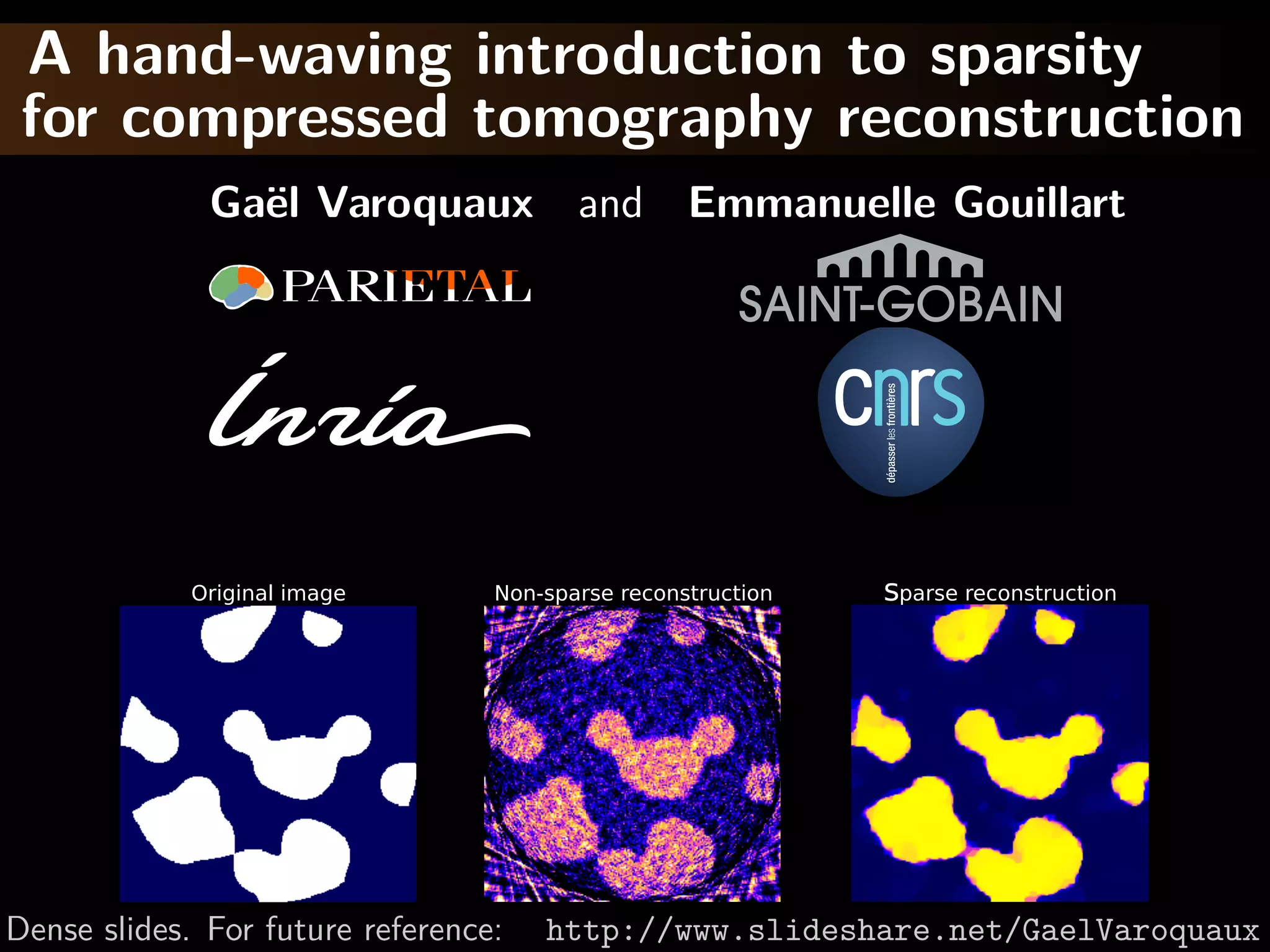
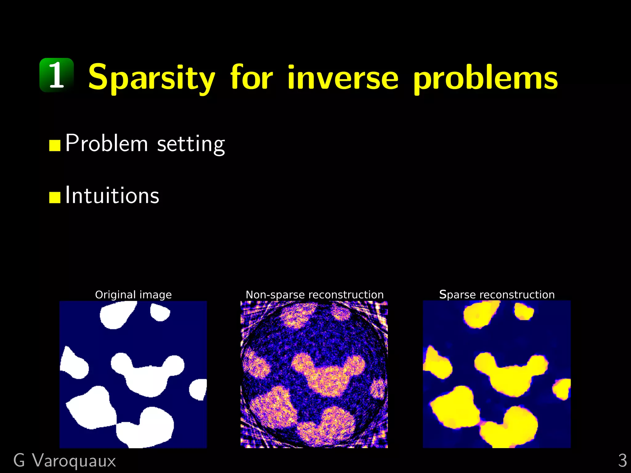
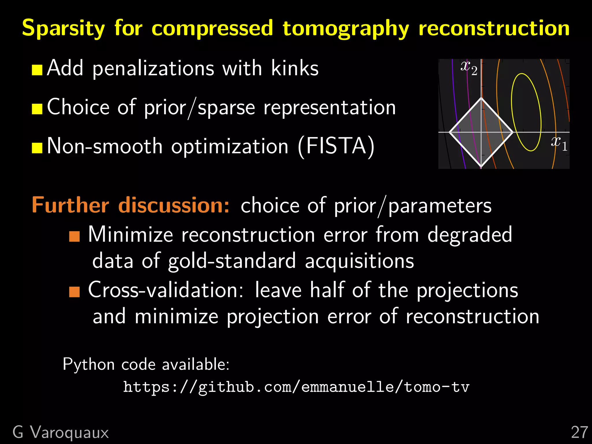
The document provides a hand-waving introduction to using sparsity for compressed tomography reconstruction. It discusses how imposing sparsity can help solve ill-posed inverse problems with limited data by finding sparse solutions. Mathematical formulations are presented using L1-norm minimization and techniques like total variation. Optimization algorithms like iterative shrinkage-thresholding are described, which use proximal operators to handle non-smooth terms in the objective function.


![Vibe Coding vs. Spec-Driven Development [Free Meetup]](https://cdn.slidesharecdn.com/ss_thumbnails/vibecodingvsspecdrivendevelopment-251209105622-43f455e7-thumbnail.jpg?width=640&height=640&fit=bounds)


