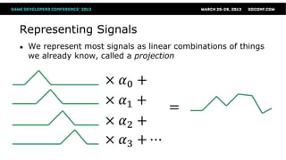
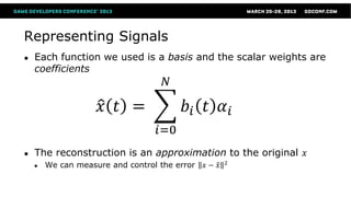
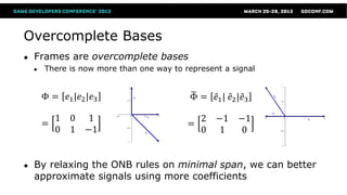
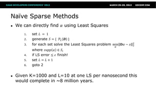
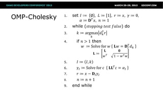
Orthogonal Matching Pursuit
and K-SVD for Sparse Encoding

Manny Ko
Senior Software Engineer, Imaginations Technologies
Robin Green
SSDE, Microsoft Xbox ATG
Outline
●   Signal Representation
●   Orthonormal Bases vs. Frames
●   Dictionaries
●   The Sparse Signal Model
●   Matching Pursuit
●   Implementing Orthonomal Matching Pursuit
●   Learned Dictionaries and KSVD
●   Image Processing with Learned Dictionaries
●   OMP for GPUs
Representing Signals
●   We represent most signals as linear combinations of things
    we already know, called a projection


                      ×    𝛼0 +
                      ×    𝛼1 +   =
                      ×    𝛼2 +
                      ×    𝛼3 + ⋯
Representing Signals
●   Each function we used is a basis and the scalar weights are
    coefficients
                                    𝑁

                     𝑥 𝑡 =               𝑏𝑖 𝑡 𝛼 𝑖
                                  𝑖=0
●   The reconstruction is an approximation to the original 𝑥
                                                      2
    ●   We can measure and control the error   𝑥− 𝑥
Orthonormal Bases (ONBs)
●   The simplest way to represent signals is using a set of
    orthonormal bases

         +∞
                                  0           𝑖≠ 𝑗
               𝑏 𝑖 𝑡 𝑏 𝑗 (𝑡) 𝑑𝑡 =
                                  1           𝑖= 𝑗
        −∞
Example ONBs
●   Fourier Basis                      ●   Gabor Functions
𝑏 𝑘 𝑡 = 𝑒 𝑖2𝑝𝑘𝑡                        𝑏 𝑘,𝑛 𝑡 = 𝜔 𝑡 − 𝑏𝑛 𝑒 𝑖2𝑝𝑘𝑡


●   Wavelets                           ●   Contourlet
𝑏   𝑚,𝑛   𝑡 = 𝑎−𝑚   2   𝑥 𝑎−𝑚 𝑡 − 𝑏𝑚   𝑏 𝑗,𝑘,𝐧 𝑡 = λ 𝑗,𝑘 𝑡 − 2 𝑗−1 𝐒 𝑘 n
Benefits of ONB
●   Analytic formulations

●   Well understood mathematical properties

●   Fast algorithms for projection
Limitations
●   Orthonormal bases are optimal only for specific synthetic
    signals
    ●   If your signal looks exactly like your basis, you only need one
        coefficient


●   Limited expressiveness, all signals behave the same

●   Real world signals often take a lot of coefficients
    ●   Just truncate the series, which leads to artifacts like aliasing
Smooth vs. Sharp
Haar Wavelet Basis   Discrete Cosine Transform
● Sharp edges        ● Smooth signals
● Local support      ● Global support
Overcomplete Bases
●   Frames are overcomplete bases
    ●   There is now more than one way to represent a signal


        Φ = 𝑒1 |𝑒2 |𝑒3                     Φ = 𝑒1 | 𝑒2 |𝑒3

            1 0 1                              2 −1    −1
        =                                  =
            0 1 −1                             0 1     0


●   By relaxing the ONB rules on minimal span, we can better
    approximate signals using more coefficients
Dictionaries
●   A dictionary is an overcomplete basis made of atoms
●   A signal is represented using a linear combination of only a
    few atoms

                           𝑑𝑖 𝛼𝑖 = 𝑥
                     𝑖∈𝐼
                            𝑫𝛼 = 𝑥

●   Atoms work best when zero-mean and normalized
Dictionaries


                       =

                           𝑥
               𝐃
                   α
Mixed Dictionaries
●   A dictionary of Haar + DCT gives the best of both worlds


    But now how do we pick which coefficients to use?
The Sparse Signal Model
                   𝐾


      𝑁                             =              𝑁


           A fixed dictionary
                                           𝑥   resulting


                   𝐃
                                                signal


                                𝛼
                                      Sparse
                                     vector of
                                    coefficients
The Sparse Signal Model
It’s Simple
 ●   Every result is built from a combination of a few atoms


It’s Rich
 ●   It’s a general model, signals are a union of many low dimensional parts


It’s Used Everywhere
 ●   The same model is used for years in Wavelets, JPEG compression,
     anything where we’ve been throwing away coefficients
Solving for Sparsity
What is the minimum number of coefficients we can use?

  1.   Sparsity Constrained
       keep adding atoms until we reach a maximum count
                                        2
             𝛼 = argmin       𝐃𝛼 − 𝑥    2    s. t.   𝛼   0   ≤ 𝐾
                      𝛼
  2.   Error Constrained
       Keep adding atoms until we reach a certain accuracy

                                                         2
             𝛼 = argmin      𝛼   0   s. t.      𝐃𝛼 − 𝑥   2   ≤ 𝜖
                      𝛼
Naïve Sparse Methods
●   We can directly find 𝛼 using Least Squares
        1.   set 𝐿 = 1
        2.   generate 𝑆 = { 𝒫 𝐿 𝑫 }
                                                                       2
        3.   for each set solve the Least Squares problem min 𝐃𝛼 − 𝑥   2
                                                           𝛼
             where 𝑠𝑢𝑝𝑝 𝛼 ∈ 𝑆 𝑖
        4.   if LS error ≤ 𝜖 finish!
        5.   set 𝐿 = 𝐿 + 1
        6.   goto 2


●   Given K=1000 and L=10 at one LS per nanosecond this
    would complete in ~8 million years.
Greedy Methods
Matching Pursuit
1. Set the residual 𝑟 = 𝑥
2. Find an unselected atom             =
   that best matches the
   residual 𝐃𝛼 − 𝑟
                                           𝑥
                               𝐃
3. Re-calculate the residual
   from matched atoms
    𝑟 = 𝑥 − 𝐃𝛼
4. Repeat until 𝑟 ≤ 𝜖
                                   𝛼
Problems with Matching Pursuit (MP)
●   If the dictionary contains atoms that are very similar, they
    tend to match the residual over and over

●   Similar atoms do not help the basis span the space of
    representable values quickly, wasting coefficients in a
    sparsity constrained solution

●   Similar atoms may match strongly but will not have a large
    effect in reducing the absolute error in an error constrained
    solution
Orthogonal Matching Pursuit (OMP)
●   Add an Orthogonal Projection to the residual calculation

    1.   set 𝐼 ∶= ∅ , 𝑟 ≔ 𝑥, 𝛾 ≔ 0
    2.   while (𝑠𝑡𝑜𝑝𝑝𝑖𝑛𝑔 𝑡𝑒𝑠𝑡 𝑓𝑎𝑙𝑠𝑒) do
    3.      𝑘 ≔ argmax 𝑑 𝑘𝑇 𝑟
                    𝑘
    4.     𝐼 ≔ 𝐼, 𝑘
    5.     𝛾𝐼 ≔ 𝐃𝐼 + 𝑥
    6.     𝑟 ≔ 𝑥 − 𝐃𝐼 𝛾𝐼
    7.   end while
Uniqueness and Stability
●   OMP has guaranteed reconstruction (provided the
    dictionary is overcomplete)

●   By projecting the input into the range-space of the atoms,
    we know that that the residual will be orthogonal to the
    selected atoms

●   Unlike Matching Pursuit (MP) that atom, and all similar
    ones, will not be reselected so more of the space is
    spanned per iteration
Orthogonal Projection
●   If the dictionary 𝐃 was square, we could use an inverse
●   Instead we use the Pseudo-inverse 𝐃+ = 𝐃 𝑇 𝐃 −1 𝐃 𝑇


                     −1
         ×    𝐃                       𝑖𝑛𝑣   ×
    𝐃𝑇                      𝐃𝑇   =              𝐃𝑇   =   𝐃+
Pseudoinverse is Fragile
                                                      −1
●   In floating point, the expression 𝐃T 𝐃   is notoriously
    numerically troublesome – the classic FP example

    ●   Picture mapping all the points on a sphere using 𝐃 𝑇 𝐃 then inverting
Implementing the Pseudoinverse
●   To avoid this, and reduce the cost of inversion, we can note that
     𝐃T 𝐃 is always symmetric and positive definite

●   We can break the matrix into two triangular matrices using Cholesky
    Decomposition 𝐀 = 𝐋𝐋 𝑇

●   Incremental Cholesky Decomp reuses the results of the previous
    iteration, adding a single new row and column each time
                      𝐋        0
            𝐋 𝑛𝑒𝑤 =                       where     𝑤 = 𝐋−1 𝐷 𝐼 𝑑 𝑘
                      𝑤𝑇    1 − 𝑤𝑇 𝑤
set 𝐼 ∶= ∅ , 𝐿 ≔ 1 , 𝑟 ≔ 𝑥, 𝛾 ≔ 0,
OMP-Cholesky   1.
                        𝛼 ≔ 𝐃 𝑇 𝑥, 𝑛 ≔ 1
               2.   while (𝑠𝑡𝑜𝑝𝑝𝑖𝑛𝑔 𝑡𝑒𝑠𝑡 𝑓𝑎𝑙𝑠𝑒) do
               3.      𝑘 ≔ argmax 𝑑 𝑘𝑇 𝑟
                               𝑘
               4.     if 𝑛 > 1 then
                          𝑤 ≔ Solve for 𝑤       𝐋𝑤 = 𝐃 𝐼𝑇 𝑑 𝑘
                                        𝐋           𝟎
                                   𝐋≔
                                        𝑤𝑇     1− 𝑤𝑇 𝑤
               5.     𝐼 ≔ 𝐼, 𝑘
               6.     𝛾 𝐼 ≔ Solve for 𝑐      𝐋𝐋 𝑇 𝑐 = 𝛼 𝐼
               7.     𝑟 ≔ 𝑥 − 𝐃𝐼 𝛾𝐼
               8.      𝑛≔ 𝑛+1
               9.   end while
OMP compression of Barbara


 2 atoms        3 atoms      4 atoms
Batch OMP (BOMP)
●   By pre-computing matrices, Batch OMP can speed up OMP
    on large numbers (>1000) of inputs against one dictionary
●   To avoid computing 𝐃 𝑇 𝑟 at each iteration

                  𝐃𝑇 𝑟 =   𝐃 𝑇 (𝑥 − 𝐃 𝐼 (𝐃 𝐈 )+ 𝑥)
                       =    𝐃 𝑇 𝑥 − 𝐆 𝐼 (𝐃 𝐼 )+ 𝑥
                       =   𝐃 𝑇 𝑥 − 𝐆 𝐼 (𝐃 𝐼𝑇 𝐃 𝐼 )−1 𝐃 𝐼𝑇 𝑥
                       =   𝐃 𝑇 𝑥 − 𝐆 𝐼 (𝐆 𝐼,𝐼 )−1 𝐃 𝐼𝑇 𝑥

●   Precompute 𝐃 𝑇 𝑥 and the Gram-matrix 𝐆 = 𝐃 𝑇 𝐃
Learned Dictionaries and K-SVD
●   OMP works well for a fixed dictionary, but it would work
    better if we could optimize the dictionary to fit the data


     𝐗   ⋯        ≈                𝐃                     𝐀⋯
Sourcing Enough Data
●   For training you will need a large number of samples
    compared to the size of the dictionary.
●   Take blocks from all integer offsets on the pixel grid


                                         𝑥=           …
𝐃
1. Sparse Encode
●   Sparse encode all entries
    in 𝐱. Collect these sparse
    vectors into a square
    array 𝐀


                                      ⋯
                                 ⋯
                                 𝐗T   𝐀T
2. Dictionary Update
●   Find all 𝐗 that use atom in
    column 𝒅 𝑘


                                      ⋯
                                  ⋯
2. Dictionary Update
●   Find all 𝐗 that use atom in
    column 𝑑 𝑘

●   Calculate the error without 𝑑 𝑘
    by 𝐄 = 𝐗 𝐼 − 𝑖≠𝑘 𝑑 𝑖 𝐀 𝐢
                                                                𝑎
●   Solve the LS problem:
                                      2
           𝑑, 𝑎 = Argmin 𝐄 − 𝑑𝑎 𝑇      𝐹   𝑠. 𝑡.   𝑑   2   =1
                       𝑑,𝑎
●   Update 𝑑 𝑖 with the new 𝑑
    and 𝐀 with the new 𝑎
Atoms after K-SVD Update
How many iterations of update?
  600000


  550000


  500000


  450000


  400000
                                                  Batch OMP
  350000


  300000                                          K-SVD
  250000


  200000
           0   10   20   30   40   50   60   70
Sparse Image Compression
●   As we have seen, we can control the number of atoms
    used per block

●   We can also specify the exact size of the dictionary and
    optimize it for each data source

●   The resulting coefficient stream can be coded using a
    Predictive Coder like Huffman or Arithmetic coding
Domain Specific Compression
●    Using just 550 bytes
     per image


1.   Original
2.   JPEG
3.   JPEG2000
4.   PCA
5.   KSVD per block
Sparse Denoising
●   Uniform noise is incompressible and OMP will reject it
●   KSVD can train a denoising dictionary from noisy image blocks


                            20
         Source            Noisy image         Result 30.829dB
Sparse Inpainting
●   Missing values in 𝐱 means missing rows in 𝐃
●   Remove these rows and refit α to recover 𝐱
    ●   If 𝛼 was sparse enough, the recovery will be perfect


                                                 =
Sparse Inpainting


  Original    80% missing   Result
Super Resolution
Super Resolution


  The Original   Bicubic Interpolation   SR result
Block compression of Voxel grids
●   “A Compression Domain output-sensitive volume rendering architecture
    based on sparse representation of voxel blocks” Gobbetti, Guitian and
    Marton [2012]

●   COVRA sparsely represents each voxel block as a dictionary of 8x8x8
    blocks and three coefficients

●   The voxel patch is reconstructed only inside the GPU shader so voxels are
    decompressed just-in-time

●   Huge bandwidth improvements, larger models and faster rendering
Thank you to:
●   Ron Rubstein & Michael Elad
●   Marc LeBrun
●   Enrico Gobbetti

omp-and-k-svd - Gdc2013

  • 1.
    Orthogonal Matching Pursuit andK-SVD for Sparse Encoding Manny Ko Senior Software Engineer, Imaginations Technologies Robin Green SSDE, Microsoft Xbox ATG
  • 2.
    Outline ● Signal Representation ● Orthonormal Bases vs. Frames ● Dictionaries ● The Sparse Signal Model ● Matching Pursuit ● Implementing Orthonomal Matching Pursuit ● Learned Dictionaries and KSVD ● Image Processing with Learned Dictionaries ● OMP for GPUs
  • 3.
    Representing Signals ● We represent most signals as linear combinations of things we already know, called a projection × 𝛼0 + × 𝛼1 + = × 𝛼2 + × 𝛼3 + ⋯
  • 4.
    Representing Signals ● Each function we used is a basis and the scalar weights are coefficients 𝑁 𝑥 𝑡 = 𝑏𝑖 𝑡 𝛼 𝑖 𝑖=0 ● The reconstruction is an approximation to the original 𝑥 2 ● We can measure and control the error 𝑥− 𝑥
  • 5.
    Orthonormal Bases (ONBs) ● The simplest way to represent signals is using a set of orthonormal bases +∞ 0 𝑖≠ 𝑗 𝑏 𝑖 𝑡 𝑏 𝑗 (𝑡) 𝑑𝑡 = 1 𝑖= 𝑗 −∞
  • 6.
    Example ONBs ● Fourier Basis ● Gabor Functions 𝑏 𝑘 𝑡 = 𝑒 𝑖2𝑝𝑘𝑡 𝑏 𝑘,𝑛 𝑡 = 𝜔 𝑡 − 𝑏𝑛 𝑒 𝑖2𝑝𝑘𝑡 ● Wavelets ● Contourlet 𝑏 𝑚,𝑛 𝑡 = 𝑎−𝑚 2 𝑥 𝑎−𝑚 𝑡 − 𝑏𝑚 𝑏 𝑗,𝑘,𝐧 𝑡 = λ 𝑗,𝑘 𝑡 − 2 𝑗−1 𝐒 𝑘 n
  • 7.
    Benefits of ONB ● Analytic formulations ● Well understood mathematical properties ● Fast algorithms for projection
  • 8.
    Limitations ● Orthonormal bases are optimal only for specific synthetic signals ● If your signal looks exactly like your basis, you only need one coefficient ● Limited expressiveness, all signals behave the same ● Real world signals often take a lot of coefficients ● Just truncate the series, which leads to artifacts like aliasing
  • 9.
    Smooth vs. Sharp HaarWavelet Basis Discrete Cosine Transform ● Sharp edges ● Smooth signals ● Local support ● Global support
  • 10.
    Overcomplete Bases ● Frames are overcomplete bases ● There is now more than one way to represent a signal Φ = 𝑒1 |𝑒2 |𝑒3 Φ = 𝑒1 | 𝑒2 |𝑒3 1 0 1 2 −1 −1 = = 0 1 −1 0 1 0 ● By relaxing the ONB rules on minimal span, we can better approximate signals using more coefficients
  • 11.
    Dictionaries ● A dictionary is an overcomplete basis made of atoms ● A signal is represented using a linear combination of only a few atoms 𝑑𝑖 𝛼𝑖 = 𝑥 𝑖∈𝐼 𝑫𝛼 = 𝑥 ● Atoms work best when zero-mean and normalized
  • 12.
    Dictionaries = 𝑥 𝐃 α
  • 13.
    Mixed Dictionaries ● A dictionary of Haar + DCT gives the best of both worlds But now how do we pick which coefficients to use?
  • 14.
    The Sparse SignalModel 𝐾 𝑁 = 𝑁 A fixed dictionary 𝑥 resulting 𝐃 signal 𝛼 Sparse vector of coefficients
  • 15.
    The Sparse SignalModel It’s Simple ● Every result is built from a combination of a few atoms It’s Rich ● It’s a general model, signals are a union of many low dimensional parts It’s Used Everywhere ● The same model is used for years in Wavelets, JPEG compression, anything where we’ve been throwing away coefficients
  • 16.
    Solving for Sparsity Whatis the minimum number of coefficients we can use? 1. Sparsity Constrained keep adding atoms until we reach a maximum count 2 𝛼 = argmin 𝐃𝛼 − 𝑥 2 s. t. 𝛼 0 ≤ 𝐾 𝛼 2. Error Constrained Keep adding atoms until we reach a certain accuracy 2 𝛼 = argmin 𝛼 0 s. t. 𝐃𝛼 − 𝑥 2 ≤ 𝜖 𝛼
  • 17.
    Naïve Sparse Methods ● We can directly find 𝛼 using Least Squares 1. set 𝐿 = 1 2. generate 𝑆 = { 𝒫 𝐿 𝑫 } 2 3. for each set solve the Least Squares problem min 𝐃𝛼 − 𝑥 2 𝛼 where 𝑠𝑢𝑝𝑝 𝛼 ∈ 𝑆 𝑖 4. if LS error ≤ 𝜖 finish! 5. set 𝐿 = 𝐿 + 1 6. goto 2 ● Given K=1000 and L=10 at one LS per nanosecond this would complete in ~8 million years.
  • 18.
    Greedy Methods Matching Pursuit 1.Set the residual 𝑟 = 𝑥 2. Find an unselected atom = that best matches the residual 𝐃𝛼 − 𝑟 𝑥 𝐃 3. Re-calculate the residual from matched atoms 𝑟 = 𝑥 − 𝐃𝛼 4. Repeat until 𝑟 ≤ 𝜖 𝛼
  • 19.
    Problems with MatchingPursuit (MP) ● If the dictionary contains atoms that are very similar, they tend to match the residual over and over ● Similar atoms do not help the basis span the space of representable values quickly, wasting coefficients in a sparsity constrained solution ● Similar atoms may match strongly but will not have a large effect in reducing the absolute error in an error constrained solution
  • 20.
    Orthogonal Matching Pursuit(OMP) ● Add an Orthogonal Projection to the residual calculation 1. set 𝐼 ∶= ∅ , 𝑟 ≔ 𝑥, 𝛾 ≔ 0 2. while (𝑠𝑡𝑜𝑝𝑝𝑖𝑛𝑔 𝑡𝑒𝑠𝑡 𝑓𝑎𝑙𝑠𝑒) do 3. 𝑘 ≔ argmax 𝑑 𝑘𝑇 𝑟 𝑘 4. 𝐼 ≔ 𝐼, 𝑘 5. 𝛾𝐼 ≔ 𝐃𝐼 + 𝑥 6. 𝑟 ≔ 𝑥 − 𝐃𝐼 𝛾𝐼 7. end while
  • 21.
    Uniqueness and Stability ● OMP has guaranteed reconstruction (provided the dictionary is overcomplete) ● By projecting the input into the range-space of the atoms, we know that that the residual will be orthogonal to the selected atoms ● Unlike Matching Pursuit (MP) that atom, and all similar ones, will not be reselected so more of the space is spanned per iteration
  • 22.
    Orthogonal Projection ● If the dictionary 𝐃 was square, we could use an inverse ● Instead we use the Pseudo-inverse 𝐃+ = 𝐃 𝑇 𝐃 −1 𝐃 𝑇 −1 × 𝐃 𝑖𝑛𝑣 × 𝐃𝑇 𝐃𝑇 = 𝐃𝑇 = 𝐃+
  • 23.
    Pseudoinverse is Fragile −1 ● In floating point, the expression 𝐃T 𝐃 is notoriously numerically troublesome – the classic FP example ● Picture mapping all the points on a sphere using 𝐃 𝑇 𝐃 then inverting
  • 24.
    Implementing the Pseudoinverse ● To avoid this, and reduce the cost of inversion, we can note that 𝐃T 𝐃 is always symmetric and positive definite ● We can break the matrix into two triangular matrices using Cholesky Decomposition 𝐀 = 𝐋𝐋 𝑇 ● Incremental Cholesky Decomp reuses the results of the previous iteration, adding a single new row and column each time 𝐋 0 𝐋 𝑛𝑒𝑤 = where 𝑤 = 𝐋−1 𝐷 𝐼 𝑑 𝑘 𝑤𝑇 1 − 𝑤𝑇 𝑤
  • 25.
    set 𝐼 ∶=∅ , 𝐿 ≔ 1 , 𝑟 ≔ 𝑥, 𝛾 ≔ 0, OMP-Cholesky 1. 𝛼 ≔ 𝐃 𝑇 𝑥, 𝑛 ≔ 1 2. while (𝑠𝑡𝑜𝑝𝑝𝑖𝑛𝑔 𝑡𝑒𝑠𝑡 𝑓𝑎𝑙𝑠𝑒) do 3. 𝑘 ≔ argmax 𝑑 𝑘𝑇 𝑟 𝑘 4. if 𝑛 > 1 then 𝑤 ≔ Solve for 𝑤 𝐋𝑤 = 𝐃 𝐼𝑇 𝑑 𝑘 𝐋 𝟎 𝐋≔ 𝑤𝑇 1− 𝑤𝑇 𝑤 5. 𝐼 ≔ 𝐼, 𝑘 6. 𝛾 𝐼 ≔ Solve for 𝑐 𝐋𝐋 𝑇 𝑐 = 𝛼 𝐼 7. 𝑟 ≔ 𝑥 − 𝐃𝐼 𝛾𝐼 8. 𝑛≔ 𝑛+1 9. end while
  • 26.
    OMP compression ofBarbara 2 atoms 3 atoms 4 atoms
  • 30.
    Batch OMP (BOMP) ● By pre-computing matrices, Batch OMP can speed up OMP on large numbers (>1000) of inputs against one dictionary ● To avoid computing 𝐃 𝑇 𝑟 at each iteration 𝐃𝑇 𝑟 = 𝐃 𝑇 (𝑥 − 𝐃 𝐼 (𝐃 𝐈 )+ 𝑥) = 𝐃 𝑇 𝑥 − 𝐆 𝐼 (𝐃 𝐼 )+ 𝑥 = 𝐃 𝑇 𝑥 − 𝐆 𝐼 (𝐃 𝐼𝑇 𝐃 𝐼 )−1 𝐃 𝐼𝑇 𝑥 = 𝐃 𝑇 𝑥 − 𝐆 𝐼 (𝐆 𝐼,𝐼 )−1 𝐃 𝐼𝑇 𝑥 ● Precompute 𝐃 𝑇 𝑥 and the Gram-matrix 𝐆 = 𝐃 𝑇 𝐃
  • 31.
    Learned Dictionaries andK-SVD ● OMP works well for a fixed dictionary, but it would work better if we could optimize the dictionary to fit the data 𝐗 ⋯ ≈ 𝐃 𝐀⋯
  • 32.
    Sourcing Enough Data ● For training you will need a large number of samples compared to the size of the dictionary. ● Take blocks from all integer offsets on the pixel grid 𝑥= …
  • 33.
    𝐃 1. Sparse Encode ● Sparse encode all entries in 𝐱. Collect these sparse vectors into a square array 𝐀 ⋯ ⋯ 𝐗T 𝐀T
  • 34.
    2. Dictionary Update ● Find all 𝐗 that use atom in column 𝒅 𝑘 ⋯ ⋯
  • 35.
    2. Dictionary Update ● Find all 𝐗 that use atom in column 𝑑 𝑘 ● Calculate the error without 𝑑 𝑘 by 𝐄 = 𝐗 𝐼 − 𝑖≠𝑘 𝑑 𝑖 𝐀 𝐢 𝑎 ● Solve the LS problem: 2 𝑑, 𝑎 = Argmin 𝐄 − 𝑑𝑎 𝑇 𝐹 𝑠. 𝑡. 𝑑 2 =1 𝑑,𝑎 ● Update 𝑑 𝑖 with the new 𝑑 and 𝐀 with the new 𝑎
  • 36.
  • 37.
    How many iterationsof update? 600000 550000 500000 450000 400000 Batch OMP 350000 300000 K-SVD 250000 200000 0 10 20 30 40 50 60 70
  • 38.
    Sparse Image Compression ● As we have seen, we can control the number of atoms used per block ● We can also specify the exact size of the dictionary and optimize it for each data source ● The resulting coefficient stream can be coded using a Predictive Coder like Huffman or Arithmetic coding
  • 40.
    Domain Specific Compression ● Using just 550 bytes per image 1. Original 2. JPEG 3. JPEG2000 4. PCA 5. KSVD per block
  • 41.
    Sparse Denoising ● Uniform noise is incompressible and OMP will reject it ● KSVD can train a denoising dictionary from noisy image blocks   20 Source Noisy image Result 30.829dB
  • 42.
    Sparse Inpainting ● Missing values in 𝐱 means missing rows in 𝐃 ● Remove these rows and refit α to recover 𝐱 ● If 𝛼 was sparse enough, the recovery will be perfect =
  • 43.
    Sparse Inpainting Original 80% missing Result
  • 44.
  • 45.
    Super Resolution The Original Bicubic Interpolation SR result
  • 46.
    Block compression ofVoxel grids ● “A Compression Domain output-sensitive volume rendering architecture based on sparse representation of voxel blocks” Gobbetti, Guitian and Marton [2012] ● COVRA sparsely represents each voxel block as a dictionary of 8x8x8 blocks and three coefficients ● The voxel patch is reconstructed only inside the GPU shader so voxels are decompressed just-in-time ● Huge bandwidth improvements, larger models and faster rendering
  • 47.
    Thank you to: ● Ron Rubstein & Michael Elad ● Marc LeBrun ● Enrico Gobbetti