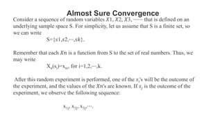
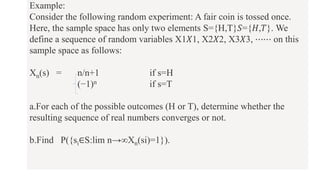
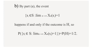
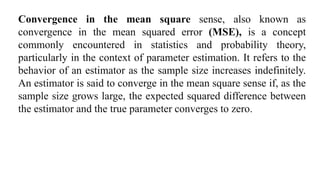
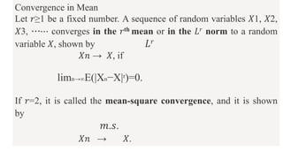
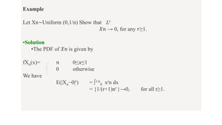
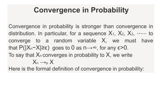
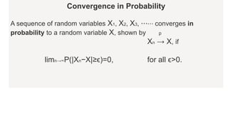
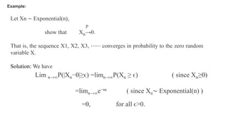
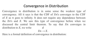
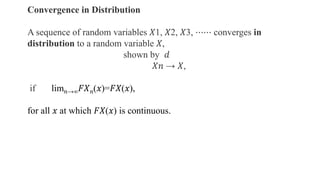
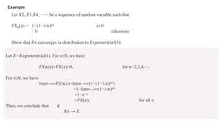
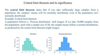
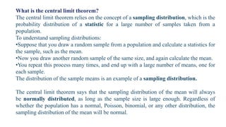
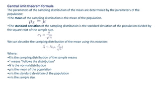
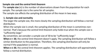
The PPT covered the distinguish between discrete and continuous distribution. Detailed explanation of the types of discrete distributions such as binomial distribution, Poisson distribution & Hyper-geometric distribution.
BINOMIAL ,POISSON AND NORMAL DISTRIBUTION.pptxletbestrong
BINOMIAL DISTRIBUTION
In probability theory and statistics, the binomial distribution is the discrete probability distribution gives only two possible results in an experiment, either Success or Failure. For example, if we toss a coin, there could be only two possible outcomes: heads or tails, and if any test is taken, then there could be only two results: pass or fail. This distribution is also called a binomial probability distribution.
Number of trials (n) is a fixed number.
The outcome of a given trial is either success or failure.
The probability of success (p) remains constant from trial to trial which means an experiment is conducted under homogeneous conditions.
The trials are independent which means the outcome of previous trial does not affect the outcome of the next trial.
Binomial Probability Distribution
In binomial probability distribution, the number of ‘Success’ in a sequence of n experiments, where each time a question is asked for yes-no, then the valued outcome is represented either with success/yes/true/one (probability p) or failure/no/false/zero (probability q = 1 − p). A single success/failure test is also called a Bernoulli trial or Bernoulli experiment, and a series of outcomes is called a Bernoulli process. For n = 1, i.e. a single experiment, the binomial distribution is a Bernoulli distribution.
There are two parameters n and p used here in a binomial distribution. The variable ‘n’ states the number of times the experiment runs and the variable ‘p’ tells the probability of any one outcome. Suppose a die is thrown randomly 10 times, then the probability of getting 2 for anyone throw is ⅙. When you throw the dice 10 times, you have a binomial distribution of n = 10 and p = ⅙.
The binomial distribution formula is for any random variable X, given by;
P(x:n,p) = nCx px (1-p)n-x
Where,
n = the number of experiments
x = 0, 1, 2, 3, 4, …
p = Probability of Success in a single experiment
q = Probability of Failure in a single experiment = 1 – p
The binomial distribution formula can also be written in the form of n-Bernoulli trials, where nCx = n!/x!(n-x)!. Hence,
P(x:n,p) = n!/[x!(n-x)!].px.(q)n-x
Binomial Distribution Mean and Variance
For a binomial distribution, the mean, variance and standard deviation for the given number of success are represented using the formulas
Mean, μ = np
Variance, σ2 = npq
Standard Deviation σ= √(npq)
Where p is the probability of success
q is the probability of failure, where q = 1-p
Properties of binomial distribution
The properties of the binomial distribution are:
• There are two possible outcomes: true or false, success or failure, yes or no.
• There is ‘n’ number of independent trials or a fixed number of n times repeated trials.
• The probability of success or failure remains the same for each trial.
• Only the number of success is calculated out of n independent trials.
• Every trial is an independent trial, which means the outcome of one trial does not affect the outcome
This 10 hours class is intended to give students the basis to empirically solve statistical problems. Talk 1 serves as an introduction to the statistical software R, and presents how to calculate basic measures such as mean, variance, correlation and gini index. Talk 2 shows how the central limit theorem and the law of the large numbers work empirically. Talk 3 presents the point estimate, the confidence interval and the hypothesis test for the most important parameters. Talk 4 introduces to the linear regression model and Talk 5 to the bootstrap world. Talk 5 also presents an easy example of a markov chains.
All the talks are supported by script codes, in R language.
In the likelihood hypothesis, a normal distribution is a sort of ceaseless likelihood conveyance for a genuine esteemed irregular variable. The overall type of its likelihood thickness work is the boundary which is the mean or desire for the circulation, while the boundary is its standard deviation.
This 10 hours class is intended to give students the basis to empirically solve statistical problems. Talk 1 serves as an introduction to the statistical software R, and presents how to calculate basic measures such as mean, variance, correlation and gini index. Talk 2 shows how the central limit theorem and the law of the large numbers work empirically. Talk 3 presents the point estimate, the confidence interval and the hypothesis test for the most important parameters. Talk 4 introduces to the linear regression model and Talk 5 to the bootstrap world. Talk 5 also presents an easy example of a markov chains.
All the talks are supported by script codes, in R language.
Lecture 5 Sampling distribution of sample mean.pptxshakirRahman10
Objectives:
Distinguish between the distribution of population and distribution of its sample means
Explain the importance of central limit
theorem
Compute and interpret the standard error of the mean.
Sampling distribution of
sample mean:
A population is a collection or a set of measurements of interest to the researcher. For example a researcher may be interested in studying the income of households in Karachi. The measurement of interest is income of each household in Karachi and the population is a list of all households in Karachi and their incomes.
Any subset of the population is called a sample from the population. A sample of ‘n’ measurements selected from a population is said to be a random sample if every different sample of size ‘n’ from the population is equally likelyto be selected.
For the purpose of estimation of certain characteristics in the population we would like to select a random sample to be a good representative of the population.
The set of measurements in the population may be summarized by a descriptive characteristic, called a parameter. In the above example the average income of households would be the parameter.
The set of measurements in a sample may be summarized by a descriptive statistic, called a statistic . For example to estimate the average household income in Karachi, we take a random sample of the population in Karachi. The sample mean is a statistic and is an estimate of the population mean.
Because no one sample is exactly like the next , the sample mean will vary from sample to sample ,and hence is itself a random variable.
Random variables have distribution ,and since the sample mean is a random variable it must have a distribution.
If the sample mean has a normal distribution ,we can compute probabilities for specific events using the properties of the normal distribution.
Consider the population with population mean = μ
and standard deviation = σ.
Next, we take many samples of size n, calculate the mean for each one of them, and create a distribution of the sample means.
This distribution is called the Sampling Distribution of Means.
Technically, a sampling distribution of a statistic is the distribution of values of the statistic in all possible samples of the same size from the same population.
Standard error of the
mean:
The quantity σ is referred to as the standard deviation .it is a measure of spread in the population .
The quality σ/n is referred to as the standard error of the sample mean .It is a measure of spread in the distribution of mean
A very important result of statistics referring to the sampling distribution of the sample mean is the Central Limit Theorem .
Central Limit Theorem:
Consider a population with finite mean and standard deviation . If random samples of n measurements are repeatedly drawn from the population then, when n is large, the relative frequency histogram for the sample means ( calculated from repeated samples)
Construction method of steel structure space frame .pptxwendy cai
High-altitude bulk installation refers to the method of total assembling of small assembled units or loose parts directly in the design position, applicable to the installation of space structure such as space frame and reticulated shell.
More Related Content
Similar to UNIT 4 PTRP final Convergence in probability.pptx
BINOMIAL ,POISSON AND NORMAL DISTRIBUTION.pptxletbestrong
BINOMIAL DISTRIBUTION
In probability theory and statistics, the binomial distribution is the discrete probability distribution gives only two possible results in an experiment, either Success or Failure. For example, if we toss a coin, there could be only two possible outcomes: heads or tails, and if any test is taken, then there could be only two results: pass or fail. This distribution is also called a binomial probability distribution.
Number of trials (n) is a fixed number.
The outcome of a given trial is either success or failure.
The probability of success (p) remains constant from trial to trial which means an experiment is conducted under homogeneous conditions.
The trials are independent which means the outcome of previous trial does not affect the outcome of the next trial.
Binomial Probability Distribution
In binomial probability distribution, the number of ‘Success’ in a sequence of n experiments, where each time a question is asked for yes-no, then the valued outcome is represented either with success/yes/true/one (probability p) or failure/no/false/zero (probability q = 1 − p). A single success/failure test is also called a Bernoulli trial or Bernoulli experiment, and a series of outcomes is called a Bernoulli process. For n = 1, i.e. a single experiment, the binomial distribution is a Bernoulli distribution.
There are two parameters n and p used here in a binomial distribution. The variable ‘n’ states the number of times the experiment runs and the variable ‘p’ tells the probability of any one outcome. Suppose a die is thrown randomly 10 times, then the probability of getting 2 for anyone throw is ⅙. When you throw the dice 10 times, you have a binomial distribution of n = 10 and p = ⅙.
The binomial distribution formula is for any random variable X, given by;
P(x:n,p) = nCx px (1-p)n-x
Where,
n = the number of experiments
x = 0, 1, 2, 3, 4, …
p = Probability of Success in a single experiment
q = Probability of Failure in a single experiment = 1 – p
The binomial distribution formula can also be written in the form of n-Bernoulli trials, where nCx = n!/x!(n-x)!. Hence,
P(x:n,p) = n!/[x!(n-x)!].px.(q)n-x
Binomial Distribution Mean and Variance
For a binomial distribution, the mean, variance and standard deviation for the given number of success are represented using the formulas
Mean, μ = np
Variance, σ2 = npq
Standard Deviation σ= √(npq)
Where p is the probability of success
q is the probability of failure, where q = 1-p
Properties of binomial distribution
The properties of the binomial distribution are:
• There are two possible outcomes: true or false, success or failure, yes or no.
• There is ‘n’ number of independent trials or a fixed number of n times repeated trials.
• The probability of success or failure remains the same for each trial.
• Only the number of success is calculated out of n independent trials.
• Every trial is an independent trial, which means the outcome of one trial does not affect the outcome
This 10 hours class is intended to give students the basis to empirically solve statistical problems. Talk 1 serves as an introduction to the statistical software R, and presents how to calculate basic measures such as mean, variance, correlation and gini index. Talk 2 shows how the central limit theorem and the law of the large numbers work empirically. Talk 3 presents the point estimate, the confidence interval and the hypothesis test for the most important parameters. Talk 4 introduces to the linear regression model and Talk 5 to the bootstrap world. Talk 5 also presents an easy example of a markov chains.
All the talks are supported by script codes, in R language.
In the likelihood hypothesis, a normal distribution is a sort of ceaseless likelihood conveyance for a genuine esteemed irregular variable. The overall type of its likelihood thickness work is the boundary which is the mean or desire for the circulation, while the boundary is its standard deviation.
This 10 hours class is intended to give students the basis to empirically solve statistical problems. Talk 1 serves as an introduction to the statistical software R, and presents how to calculate basic measures such as mean, variance, correlation and gini index. Talk 2 shows how the central limit theorem and the law of the large numbers work empirically. Talk 3 presents the point estimate, the confidence interval and the hypothesis test for the most important parameters. Talk 4 introduces to the linear regression model and Talk 5 to the bootstrap world. Talk 5 also presents an easy example of a markov chains.
All the talks are supported by script codes, in R language.
Lecture 5 Sampling distribution of sample mean.pptxshakirRahman10
Objectives:
Distinguish between the distribution of population and distribution of its sample means
Explain the importance of central limit
theorem
Compute and interpret the standard error of the mean.
Sampling distribution of
sample mean:
A population is a collection or a set of measurements of interest to the researcher. For example a researcher may be interested in studying the income of households in Karachi. The measurement of interest is income of each household in Karachi and the population is a list of all households in Karachi and their incomes.
Any subset of the population is called a sample from the population. A sample of ‘n’ measurements selected from a population is said to be a random sample if every different sample of size ‘n’ from the population is equally likelyto be selected.
For the purpose of estimation of certain characteristics in the population we would like to select a random sample to be a good representative of the population.
The set of measurements in the population may be summarized by a descriptive characteristic, called a parameter. In the above example the average income of households would be the parameter.
The set of measurements in a sample may be summarized by a descriptive statistic, called a statistic . For example to estimate the average household income in Karachi, we take a random sample of the population in Karachi. The sample mean is a statistic and is an estimate of the population mean.
Because no one sample is exactly like the next , the sample mean will vary from sample to sample ,and hence is itself a random variable.
Random variables have distribution ,and since the sample mean is a random variable it must have a distribution.
If the sample mean has a normal distribution ,we can compute probabilities for specific events using the properties of the normal distribution.
Consider the population with population mean = μ
and standard deviation = σ.
Next, we take many samples of size n, calculate the mean for each one of them, and create a distribution of the sample means.
This distribution is called the Sampling Distribution of Means.
Technically, a sampling distribution of a statistic is the distribution of values of the statistic in all possible samples of the same size from the same population.
Standard error of the
mean:
The quantity σ is referred to as the standard deviation .it is a measure of spread in the population .
The quality σ/n is referred to as the standard error of the sample mean .It is a measure of spread in the distribution of mean
A very important result of statistics referring to the sampling distribution of the sample mean is the Central Limit Theorem .
Central Limit Theorem:
Consider a population with finite mean and standard deviation . If random samples of n measurements are repeatedly drawn from the population then, when n is large, the relative frequency histogram for the sample means ( calculated from repeated samples)
Construction method of steel structure space frame .pptxwendy cai
High-altitude bulk installation refers to the method of total assembling of small assembled units or loose parts directly in the design position, applicable to the installation of space structure such as space frame and reticulated shell.
Welcome to WIPAC Monthly the magazine brought to you by the LinkedIn Group Water Industry Process Automation & Control.
In this month's edition, along with this month's industry news to celebrate the 13 years since the group was created we have articles including
A case study of the used of Advanced Process Control at the Wastewater Treatment works at Lleida in Spain
A look back on an article on smart wastewater networks in order to see how the industry has measured up in the interim around the adoption of Digital Transformation in the Water Industry.
Toll tax management system project report..pdfKamal Acharya
Toll Tax Management System is a web based application that can provide all the information related to toll plazas and the passenger checks in and pays the amount, then he/she will be provided by a receipt. With this receipt he/she can leave the toll booth without waiting for any verification call.
The information would also cover registration of staff, toll plaza collection, toll plaza collection entry for vehicles, date wise report entry, Vehicle passes and passes reports b/w dates.
Hybrid optimization of pumped hydro system and solar- Engr. Abdul-Azeez.pdffxintegritypublishin
Advancements in technology unveil a myriad of electrical and electronic breakthroughs geared towards efficiently harnessing limited resources to meet human energy demands. The optimization of hybrid solar PV panels and pumped hydro energy supply systems plays a pivotal role in utilizing natural resources effectively. This initiative not only benefits humanity but also fosters environmental sustainability. The study investigated the design optimization of these hybrid systems, focusing on understanding solar radiation patterns, identifying geographical influences on solar radiation, formulating a mathematical model for system optimization, and determining the optimal configuration of PV panels and pumped hydro storage. Through a comparative analysis approach and eight weeks of data collection, the study addressed key research questions related to solar radiation patterns and optimal system design. The findings highlighted regions with heightened solar radiation levels, showcasing substantial potential for power generation and emphasizing the system's efficiency. Optimizing system design significantly boosted power generation, promoted renewable energy utilization, and enhanced energy storage capacity. The study underscored the benefits of optimizing hybrid solar PV panels and pumped hydro energy supply systems for sustainable energy usage. Optimizing the design of solar PV panels and pumped hydro energy supply systems as examined across diverse climatic conditions in a developing country, not only enhances power generation but also improves the integration of renewable energy sources and boosts energy storage capacities, particularly beneficial for less economically prosperous regions. Additionally, the study provides valuable insights for advancing energy research in economically viable areas. Recommendations included conducting site-specific assessments, utilizing advanced modeling tools, implementing regular maintenance protocols, and enhancing communication among system components.
This document is by explosives industry in which document discussed manufacturing process and flow charts details by nitric acid and sulfuric acid and tetra benzene and step by step details of explosive industry explosives industry is produced raw materials and manufacture it by manufacturing process
Automobile Management System Project Report.pdfKamal Acharya
The proposed project is developed to manage the automobile in the automobile dealer company. The main module in this project is login, automobile management, customer management, sales, complaints and reports. The first module is the login. The automobile showroom owner should login to the project for usage. The username and password are verified and if it is correct, next form opens. If the username and password are not correct, it shows the error message.
When a customer search for a automobile, if the automobile is available, they will be taken to a page that shows the details of the automobile including automobile name, automobile ID, quantity, price etc. “Automobile Management System” is useful for maintaining automobiles, customers effectively and hence helps for establishing good relation between customer and automobile organization. It contains various customized modules for effectively maintaining automobiles and stock information accurately and safely.
When the automobile is sold to the customer, stock will be reduced automatically. When a new purchase is made, stock will be increased automatically. While selecting automobiles for sale, the proposed software will automatically check for total number of available stock of that particular item, if the total stock of that particular item is less than 5, software will notify the user to purchase the particular item.
Also when the user tries to sale items which are not in stock, the system will prompt the user that the stock is not enough. Customers of this system can search for a automobile; can purchase a automobile easily by selecting fast. On the other hand the stock of automobiles can be maintained perfectly by the automobile shop manager overcoming the drawbacks of existing system.
Natalia Rutkowska - BIM School Course in Krakówbim.edu.pl
Teaching effects after 128 hours of Building Information Modeling course in Cracow, Poland. Natalia works in Revit, Navisworks and Dynamo for BIM Coordination position. More https://bim.edu.pl or https://bimedu.eu
Final project report on grocery store management system..pdfKamal Acharya
In today’s fast-changing business environment, it’s extremely important to be able to respond to client needs in the most effective and timely manner. If your customers wish to see your business online and have instant access to your products or services.
Online Grocery Store is an e-commerce website, which retails various grocery products. This project allows viewing various products available enables registered users to purchase desired products instantly using Paytm, UPI payment processor (Instant Pay) and also can place order by using Cash on Delivery (Pay Later) option. This project provides an easy access to Administrators and Managers to view orders placed using Pay Later and Instant Pay options.
In order to develop an e-commerce website, a number of Technologies must be studied and understood. These include multi-tiered architecture, server and client-side scripting techniques, implementation technologies, programming language (such as PHP, HTML, CSS, JavaScript) and MySQL relational databases. This is a project with the objective to develop a basic website where a consumer is provided with a shopping cart website and also to know about the technologies used to develop such a website.
This document will discuss each of the underlying technologies to create and implement an e- commerce website.
A CASE STUDY ON ONLINE TICKET BOOKING SYSTEM PROJECT.pdfKamal Acharya
Online movie ticket booking system for movies is a web-based program. This application allows users to purchase cinema tickets over the portal. To buy tickets, people must first register or log in. This website's backend is PHP and JavaScript, and the front end is HTML and CSS. All phases of the software development life cycle are efficiently managed in order to design and implement software. On the website, there are two panels: one for administrators and one for customers/users. The admin has the ability to add cinemas, movies, delete, halt execution, and add screens, among other things. The website is simple to navigate and appealing, saving the end user time.
About
Indigenized remote control interface card suitable for MAFI system CCR equipment. Compatible for IDM8000 CCR. Backplane mounted serial and TCP/Ethernet communication module for CCR remote access. IDM 8000 CCR remote control on serial and TCP protocol.
• Remote control: Parallel or serial interface.
• Compatible with MAFI CCR system.
• Compatible with IDM8000 CCR.
• Compatible with Backplane mount serial communication.
• Compatible with commercial and Defence aviation CCR system.
• Remote control system for accessing CCR and allied system over serial or TCP.
• Indigenized local Support/presence in India.
• Easy in configuration using DIP switches.
Technical Specifications
Indigenized remote control interface card suitable for MAFI system CCR equipment. Compatible for IDM8000 CCR. Backplane mounted serial and TCP/Ethernet communication module for CCR remote access. IDM 8000 CCR remote control on serial and TCP protocol.
Key Features
Indigenized remote control interface card suitable for MAFI system CCR equipment. Compatible for IDM8000 CCR. Backplane mounted serial and TCP/Ethernet communication module for CCR remote access. IDM 8000 CCR remote control on serial and TCP protocol.
• Remote control: Parallel or serial interface
• Compatible with MAFI CCR system
• Copatiable with IDM8000 CCR
• Compatible with Backplane mount serial communication.
• Compatible with commercial and Defence aviation CCR system.
• Remote control system for accessing CCR and allied system over serial or TCP.
• Indigenized local Support/presence in India.
Application
• Remote control: Parallel or serial interface.
• Compatible with MAFI CCR system.
• Compatible with IDM8000 CCR.
• Compatible with Backplane mount serial communication.
• Compatible with commercial and Defence aviation CCR system.
• Remote control system for accessing CCR and allied system over serial or TCP.
• Indigenized local Support/presence in India.
• Easy in configuration using DIP switches.
Water scarcity is the lack of fresh water resources to meet the standard water demand. There are two type of water scarcity. One is physical. The other is economic water scarcity.
Event Management System Vb Net Project Report.pdfKamal Acharya
In present era, the scopes of information technology growing with a very fast .We do not see any are untouched from this industry. The scope of information technology has become wider includes: Business and industry. Household Business, Communication, Education, Entertainment, Science, Medicine, Engineering, Distance Learning, Weather Forecasting. Carrier Searching and so on.
My project named “Event Management System” is software that store and maintained all events coordinated in college. It also helpful to print related reports. My project will help to record the events coordinated by faculties with their Name, Event subject, date & details in an efficient & effective ways.
In my system we have to make a system by which a user can record all events coordinated by a particular faculty. In our proposed system some more featured are added which differs it from the existing system such as security.
Q.1 A single plate clutch with both sides of the plate effective is required to transmit 25 kW at 1600 r.p.m. The outer diameter of the plate is limited to 300 mm and the intensity of pressure between the plates not to exceed 0.07N / m * m ^ 2 Assuming uniform wear and coefficient of friction 0.3, find the inner diameter of the plates and the axial force necessary to engage the clutch.
Q.2 A multiple disc clutch has radial width of the friction material as 1/5th of the maximum radius. The coefficient of friction is 0.25. Find the total number of discs required to transmit 60 kW at 3000 r.p.m. The maximum diameter of the clutch is 250 mm and the axial force is limited to 600 N. Also find the mean unit pressure on each contact surface.
Q.3 A cone clutch is to be designed to transmit 7.5 kW at 900 r.p.m. The cone has a face angle of 12°. The width of the face is half of the mean radius and the normal pressure between the contact faces is not to exceed 0.09 N/mm². Assuming uniform wear and the coefficient of friction between the contact faces as 0.2, find the main dimensions of the clutch and the axial force required to engage the clutch.
Q.4 A cone clutch is mounted on a shaft which transmits power at 225 r.p.m. The small diameter of the cone is 230 mm, the cone face is 50 mm and the cone face makes an angle of 15 deg with the horizontal. Determine the axial force necessary to engage the clutch to transmit 4.5 kW if the coefficient of friction of the contact surfaces is 0.25. What is the maximum pressure on the contact surfaces assuming uniform wear?
Q.5 A soft surface cone clutch transmits a torque of 200 N-m at 1250 r.p.m. The larger diameter of the clutch is 350 mm. The cone pitch angle is 7.5 deg and the face width is 65 mm. If the coefficient of friction is 0.2. find:
1. the axial force required to transmit the torque:
2. the axial force required to engage the clutch;
3. the average normal pressure on the contact surfaces when the maximum torque is being transmitted; and
4. the maximum normal pressure assuming uniform wear.
Q.6 A single block brake, as shown in Fig. 1. has the drum diameter 250 mm. The angle of contact is 90° and the coefficient of friction between the drum and the lining is 0.35. If the torque transmitted by the brake is 70 N-m, find the force P required to operate the brake. Q.7 The layout and dimensions of a double shoe brake is shown in Fig. 2. The diameter of the
brake drum is 300 mm and the contact angle for each shoe is 90°. If the coefficient of friction for the brake lining and the drum is 0.4, find the spring force necessary to transmit a torque of 30 N-m. Also determine the width of the brake shoes, if the bearing pressure on the lining material is not to exceed 0.28N / m * m ^ 2
2. Almost Sure Convergence
Consider a sequence of random variables 𝑋1, 𝑋2, 𝑋3, ⋯⋯ that is defined on an
underlying sample space S. For simplicity, let us assume that S is a finite set, so
we can write
S={𝑠1,𝑠2,⋯,𝑠𝑘}.
Remember that each 𝑋𝑛 is a function from S to the set of real numbers. Thus, we
may write
Xn(si)=xni, for i=1,2,⋯,k.
After this random experiment is performed, one of the 𝑠𝑖's will be the outcome of
the experiment, and the values of the 𝑋𝑛's are known. If 𝑠𝑗 is the outcome of the
experiment, we observe the following sequence:
x1j, x2j, x3j,⋯.
3. Example:
Consider the following random experiment: A fair coin is tossed once.
Here, the sample space has only two elements S={H,T}𝑆={𝐻,𝑇}. We
define a sequence of random variables X1𝑋1, X2𝑋2, X3𝑋3, ⋯⋯ on this
sample space as follows:
Xn(s) = n/n+1 if s=H
(−1)n if s=T
a.For each of the possible outcomes (H or T), determine whether the
resulting sequence of real numbers converges or not.
b.Find P({si∈S:lim n→∞Xn(si)=1}).
4. Solution a.
If the outcome is H, then we have Xn(H)=n/n+1, so we obtain the following
sequence
1/2,2/3,3/4,4/5,⋯.
This sequence converges to 1 as n goes to infinity. If the outcome is T, then we
have
Xn(T) = (−1)n,
so we obtain the following sequence
−1,1,−1,1,−1,⋯.
5. b) By part (a), the event
{si ∈S :lim n→∞ Xn(si)=1
happens if and only if the outcome is H, so
P({si ∈ S: limn→∞ Xn(si)=1})=P(H)=1/2.
7. Convergence in the mean square sense, also known as
convergence in the mean squared error (MSE), is a concept
commonly encountered in statistics and probability theory,
particularly in the context of parameter estimation. It refers to the
behavior of an estimator as the sample size increases indefinitely.
An estimator is said to converge in the mean square sense if, as the
sample size grows large, the expected squared difference between
the estimator and the true parameter converges to zero.
8. Convergence in Mean
Let 𝑟≥1 be a fixed number. A sequence of random variables 𝑋1, 𝑋2,
𝑋3, ⋯⋯ converges in the 𝑟th mean or in the 𝐿𝑟 norm to a random
variable 𝑋, shown by 𝐿𝑟
𝑋𝑛 → 𝑋, if
limn→∞E(|Xn−X|r)=0.
If 𝑟=2, it is called the mean-square convergence, and it is shown
by
𝑚.𝑠.
𝑋𝑛 → 𝑋.
9. Example
Let Xn∼Uniform (0,1/n) Show that 𝐿𝑟
𝑋𝑛 → 0, for any 𝑟≥1.
•Solution
•The PDF of 𝑋𝑛 is given by
fXn(x)= 𝑛 0≤𝑥≤1
0 otherwise
We have
E(|Xn−0|r) = ∫1/n
0 xrn dx
= {1/(r+1)nr }→0, for all r≥1.
10. Convergence in Probability
Convergence in probability is stronger than convergence in
distribution. In particular, for a sequence X1, X2, X3, ⋯⋯ to
converge to a random variable X, we must have
that P(|Xn−X|≥ϵ) goes to 0 as n→∞, for any ϵ>0.
To say that Xn converges in probability to X, we write
Xn →p X
Here is the formal definition of convergence in probability:
11. Convergence in Probability
A sequence of random variables X1, X2, X3, ⋯⋯ converges in
probability to a random variable X, shown by p
Xn → X, if
limn→∞P(|Xn−X|≥ϵ)=0, for all ϵ>0.
12. Example:
Let Xn ∼ Exponential(n),
p
show that Xn→0.
That is, the sequence X1, X2, X3, ⋯⋯ converges in probability to the zero random
variable X.
Solution: We have
Lim n→∞P(|Xn−0|≥ϵ) =limn→∞P(Xn ≥ ϵ) ( since Xn≥0)
=limn→∞e−nϵ ( since Xn∼ Exponential(n) )
=0, for all ϵ>0.
13. Convergence in Distribution
Convergence in distribution is in some sense the weakest type of
convergence. All it says is that the CDF of 𝑋𝑛's converges to the CDF
of 𝑋 as 𝑛 goes to infinity. It does not require any dependence between
the 𝑋𝑛's and 𝑋. We saw this type of convergence before when we
discussed the central limit theorem. To say that 𝑋𝑛 converges in
distribution to 𝑋, we write 𝑑
𝑋𝑛 → 𝑋.
Here is a formal definition of convergence in distribution:
14. Convergence in Distribution
A sequence of random variables 𝑋1, 𝑋2, 𝑋3, ⋯⋯ converges in
distribution to a random variable 𝑋,
shown by 𝑑
𝑋𝑛 → 𝑋,
if lim𝑛→∞𝐹𝑋𝑛(𝑥)=𝐹𝑋(𝑥),
for all 𝑥 at which 𝐹𝑋(𝑥) is continuous.
15. Example
Let 𝑋2, 𝑋3,𝑋4, ⋯⋯ be a sequence of random variable such that
𝐹𝑋𝑛(𝑥) = 1−(1−1/𝑛)𝑛𝑥 𝑥>0
0 otherwise
Show that 𝑋𝑛 converges in distribution to 𝐸𝑥𝑝𝑜𝑛𝑒𝑛𝑡𝑖𝑎𝑙(1).
Let 𝑋∼𝐸𝑥𝑝𝑜𝑛𝑒𝑛𝑡𝑖𝑎𝑙(1). For 𝑥≤0, we have
𝐹𝑋𝑛(𝑥)=𝐹𝑋(𝑥)=0, for 𝑛=2,3,4,⋯.
For 𝑥≥0, we have
lim𝑛→∞𝐹𝑋𝑛(𝑥)=lim𝑛→∞(1−(1−1/𝑛)𝑛𝑥)
=1−lim𝑛→∞(1−1/𝑛)𝑛𝑥
=1−𝑒−𝑥
=𝐹𝑋(𝑥), for all 𝑥.
Thus, we conclude that 𝑑
𝑋𝑛 → 𝑋.
16. Central limit theorem and its significance
The central limit theorem states that if you take sufficiently large samples from a
population, the samples’ means will be normally distributed, even if the population isn’t
normally distributed.
Example: Central limit theorem
A population follows a Poisson distribution (left image). If we take 10,000 samples from
the population, each with a sample size of 50, the sample means follow a normal distribution,
as predicted by the central limit theorem (right image).
17. What is the central limit theorem?
The central limit theorem relies on the concept of a sampling distribution, which is the
probability distribution of a statistic for a large number of samples taken from a
population.
To understand sampling distributions:
•Suppose that you draw a random sample from a population and calculate a statistics for
the sample, such as the mean.
•Now you draw another random sample of the same size, and again calculate the mean.
•You repeat this process many times, and end up with a large number of means, one for
each sample.
The distribution of the sample means is an example of a sampling distribution.
The central limit theorem says that the sampling distribution of the mean will always
be normally distributed, as long as the sample size is large enough. Regardless of
whether the population has a normal, Poisson, binomial, or any other distribution, the
sampling distribution of the mean will be normal.
18. Central limit theorem formula
The parameters of the sampling distribution of the mean are determined by the parameters of the
population:
•The mean of the sampling distribution is the mean of the population.
•The standard deviation of the sampling distribution is the standard deviation of the population divided by
the square root of the sample size.
We can describe the sampling distribution of the mean using this notation:
Where:
•X̄ is the sampling distribution of the sample means
•~ means “follows the distribution”
•N is the normal distribution
•µ is the mean of the population
•σ is the standard deviation of the population
•n is the sample size
19. Sample size and the central limit theorem
The sample size (n) is the number of observations drawn from the population for each
sample. The sample size is the same for all samples.
The sample size affects the sampling distribution of the mean in two ways.
1. Sample size and normality
The larger the sample size, the more closely the sampling distribution will follow a normal
distribution.
When the sample size is small, the sampling distribution of the mean is sometimes non-
normal. That’s because the central limit theorem only holds true when the sample size is
“sufficiently large.”
By convention, we consider a sample size of 30 to be “sufficiently large.”
When n < 30, the central limit theorem doesn’t apply. The sampling distribution will follow a
similar distribution to the population. Therefore, the sampling distribution will only be
normal if the population is normal.
When n ≥ 30, the central limit theorem applies. The sampling distribution will approximately
follow a normal distribution.
20. 2. Sample size and standard deviations
The sample size affects the standard deviation of the sampling distribution.
Standard deviation is a measure of the variability or spread of the distribution
(i.e., how wide or narrow it is).
When n is low, the standard deviation is high. There’s a lot of spread in the
samples’ means because they aren’t precise estimates of the population’s
mean.
When n is high, the standard deviation is low. There’s not much spread in the
samples’ means because they’re precise estimates of the population’s mean.
21. Conditions of the central limit theorem
The central limit theorem states that the sampling distribution of the mean
will always follow a normal distribution under the following conditions:
The sample size is sufficiently large. This condition is usually met if the
sample size is n ≥ 30.
The samples are independent and identically distributed (i.i.d.) random
variables. This condition is usually met if the sampling is random.
The population’s distribution has finite variance. Central limit theorem
doesn’t apply to distributions with infinite variance, such as the Cauchy
distribution. Most distributions have finite variance.