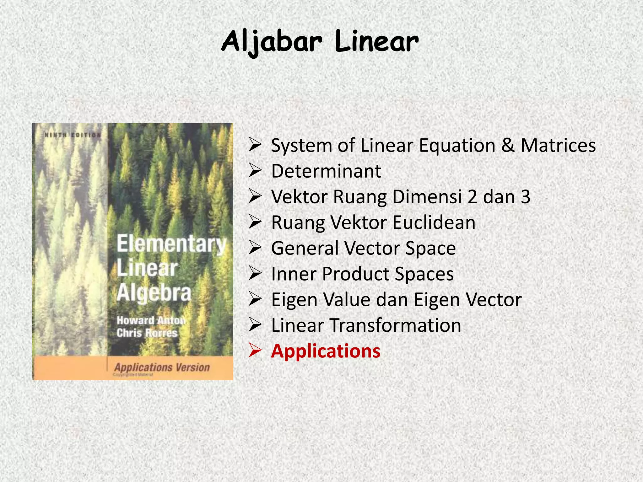
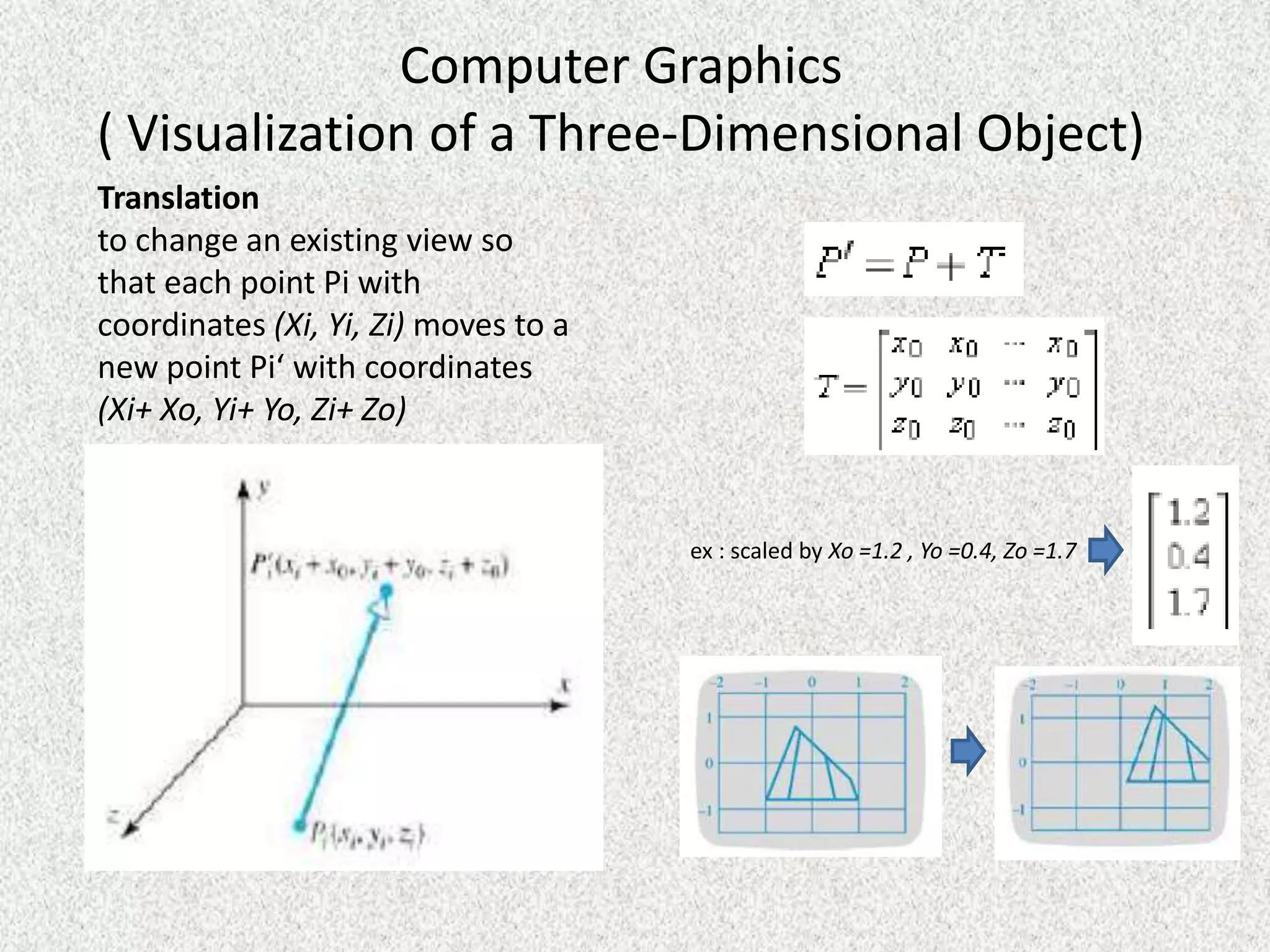
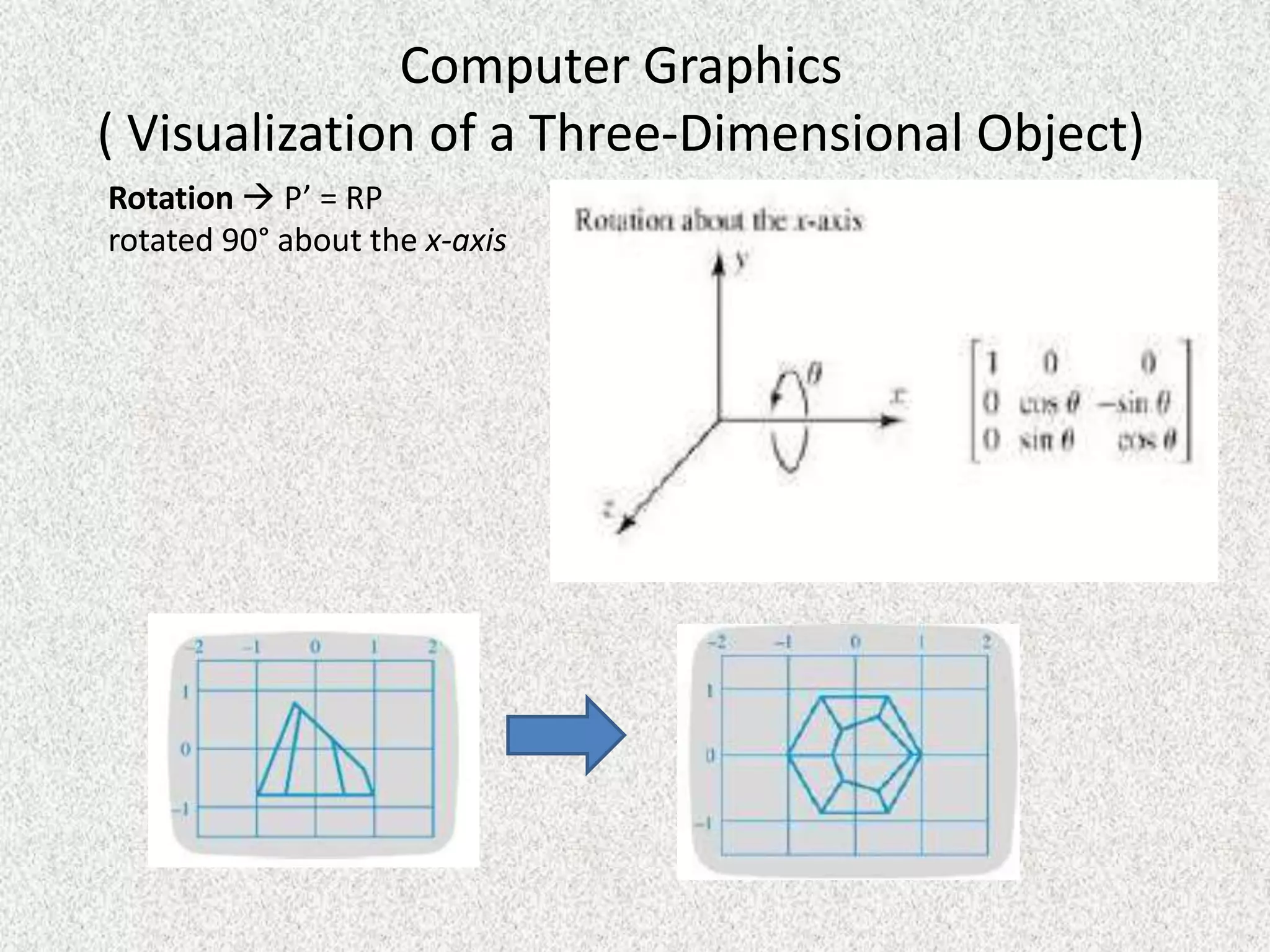
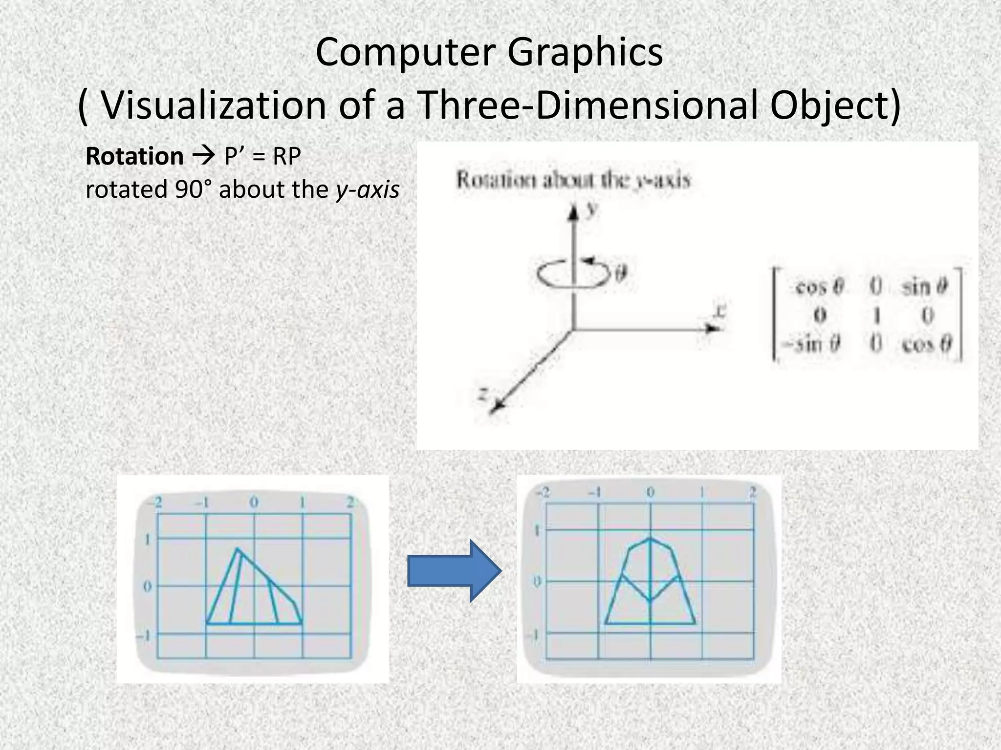
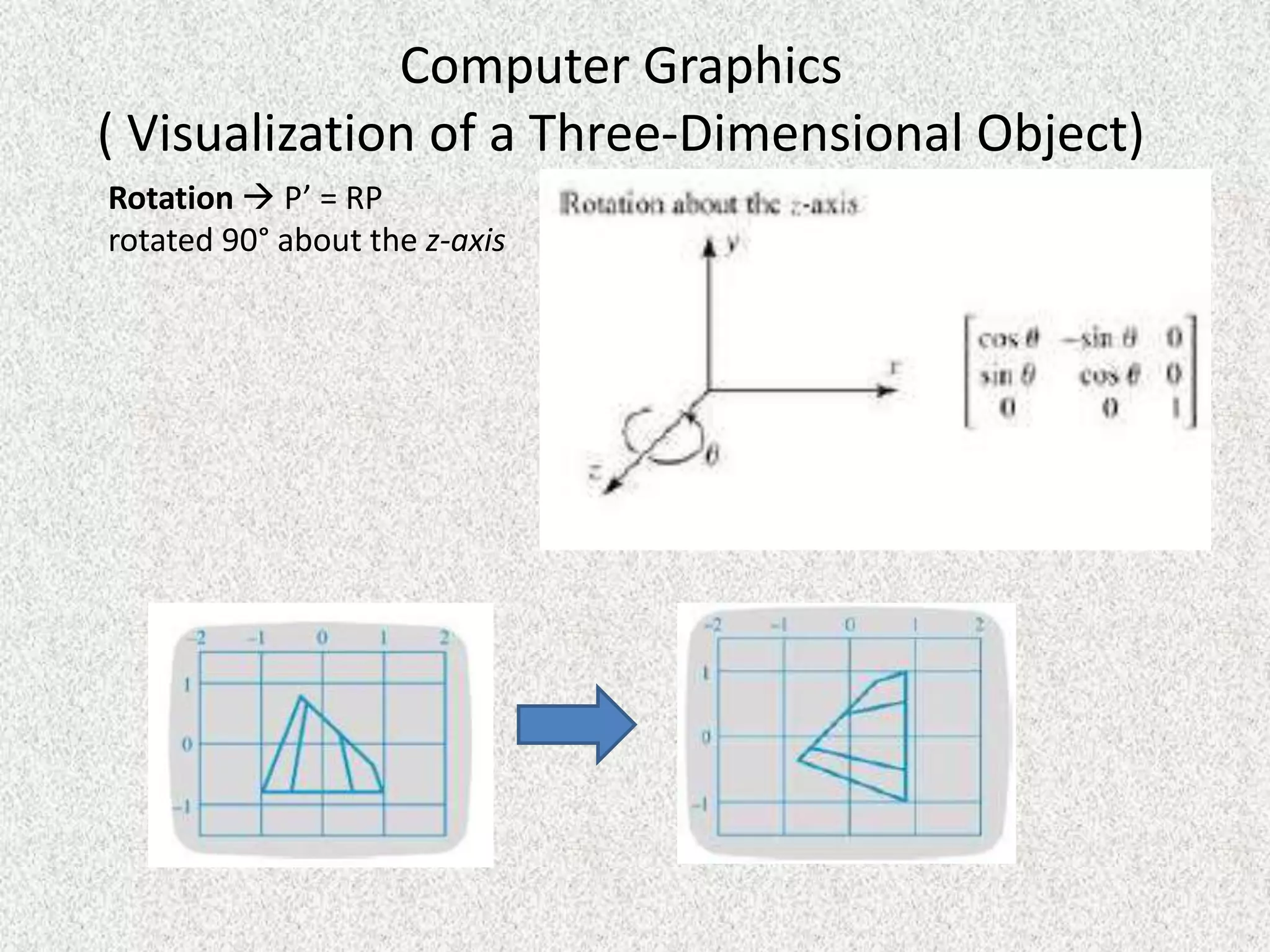
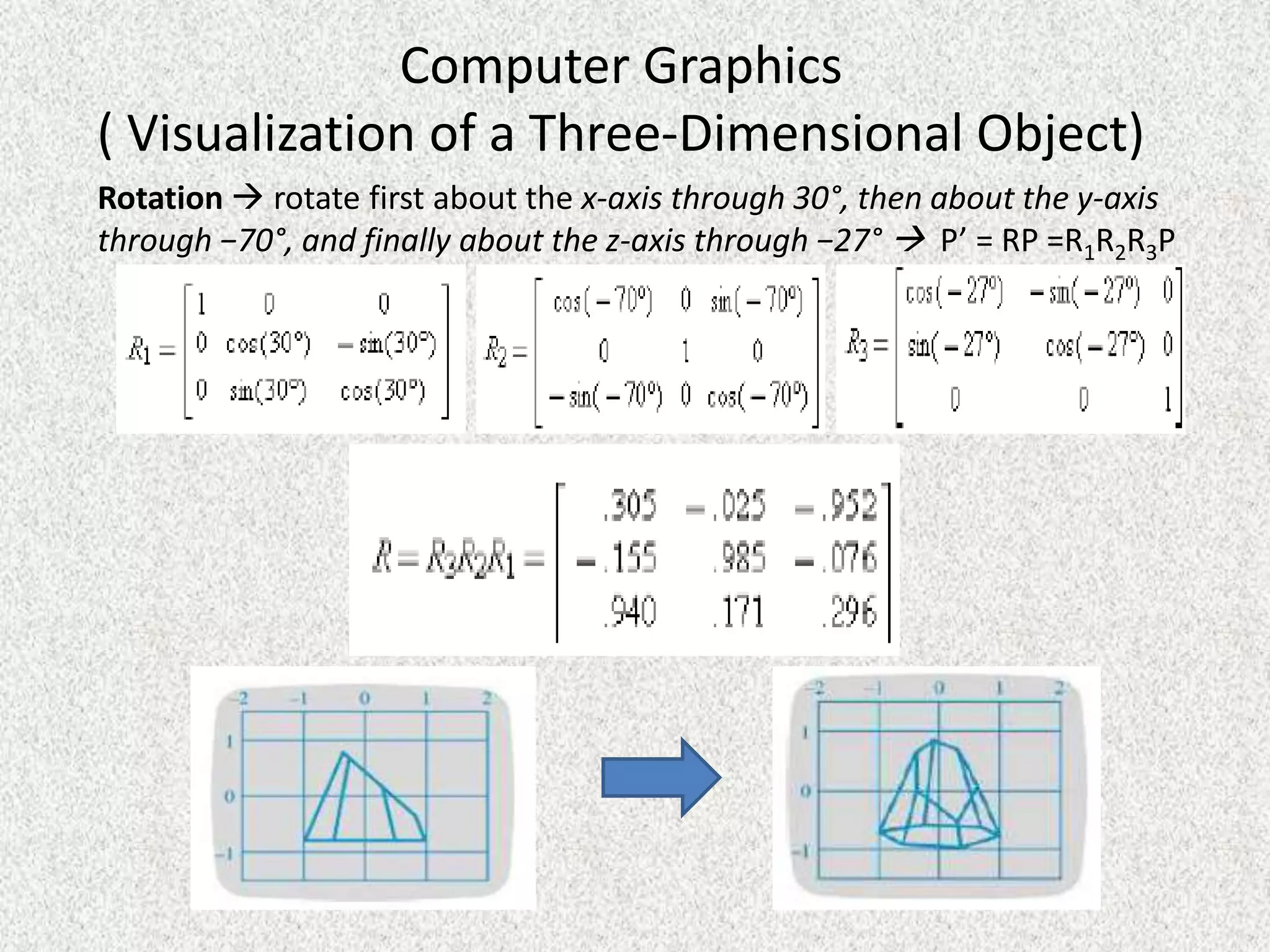
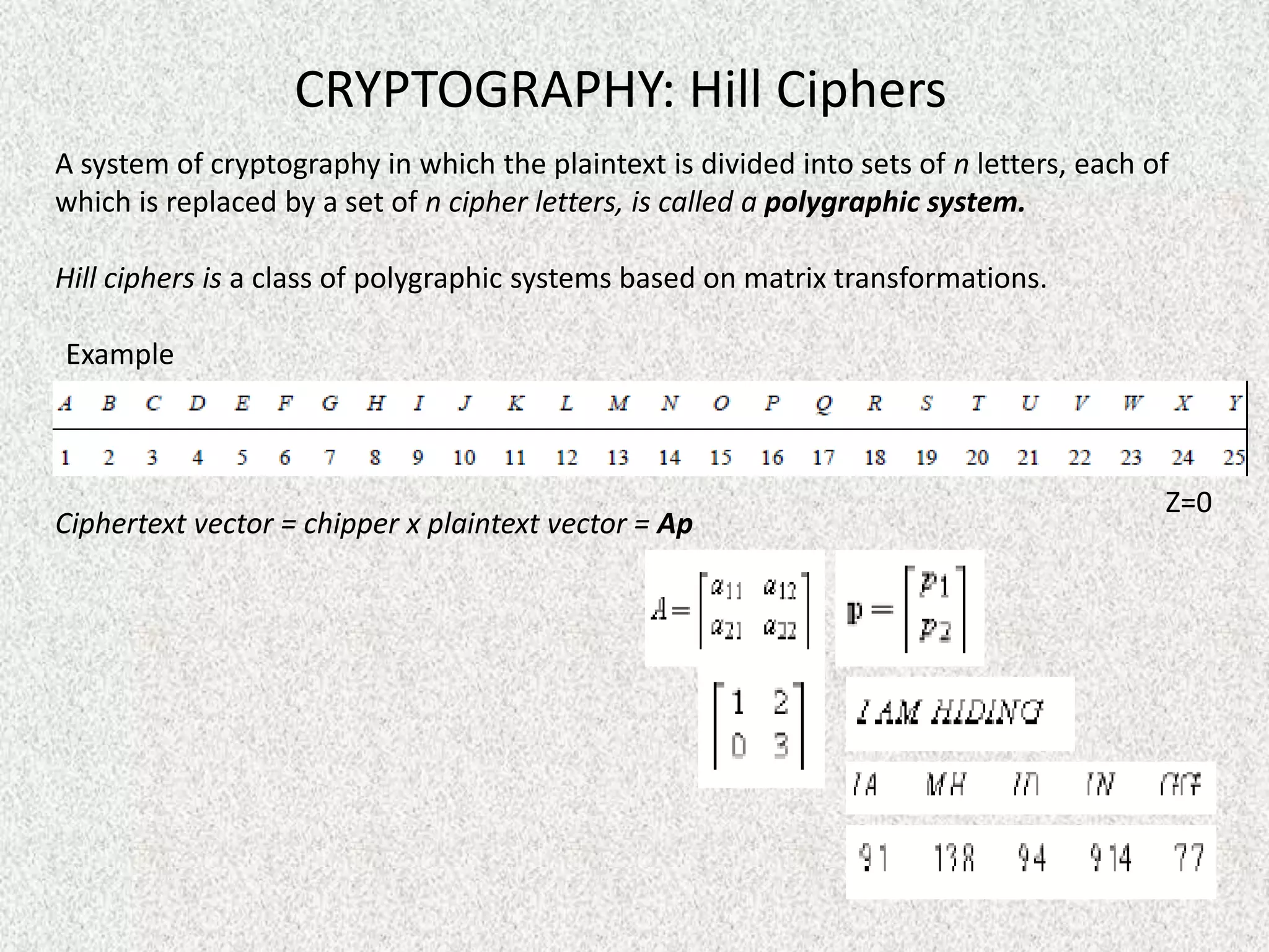
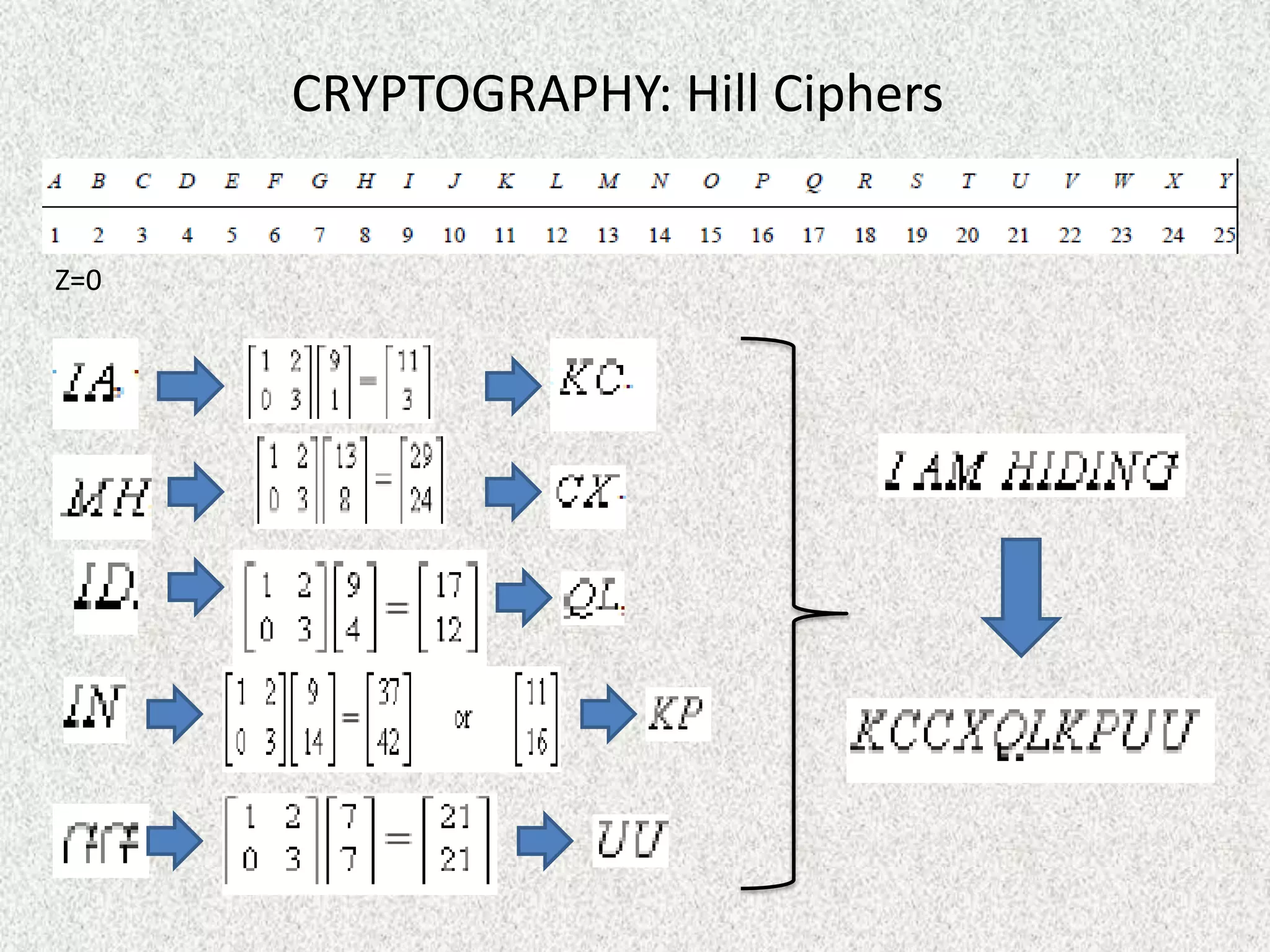
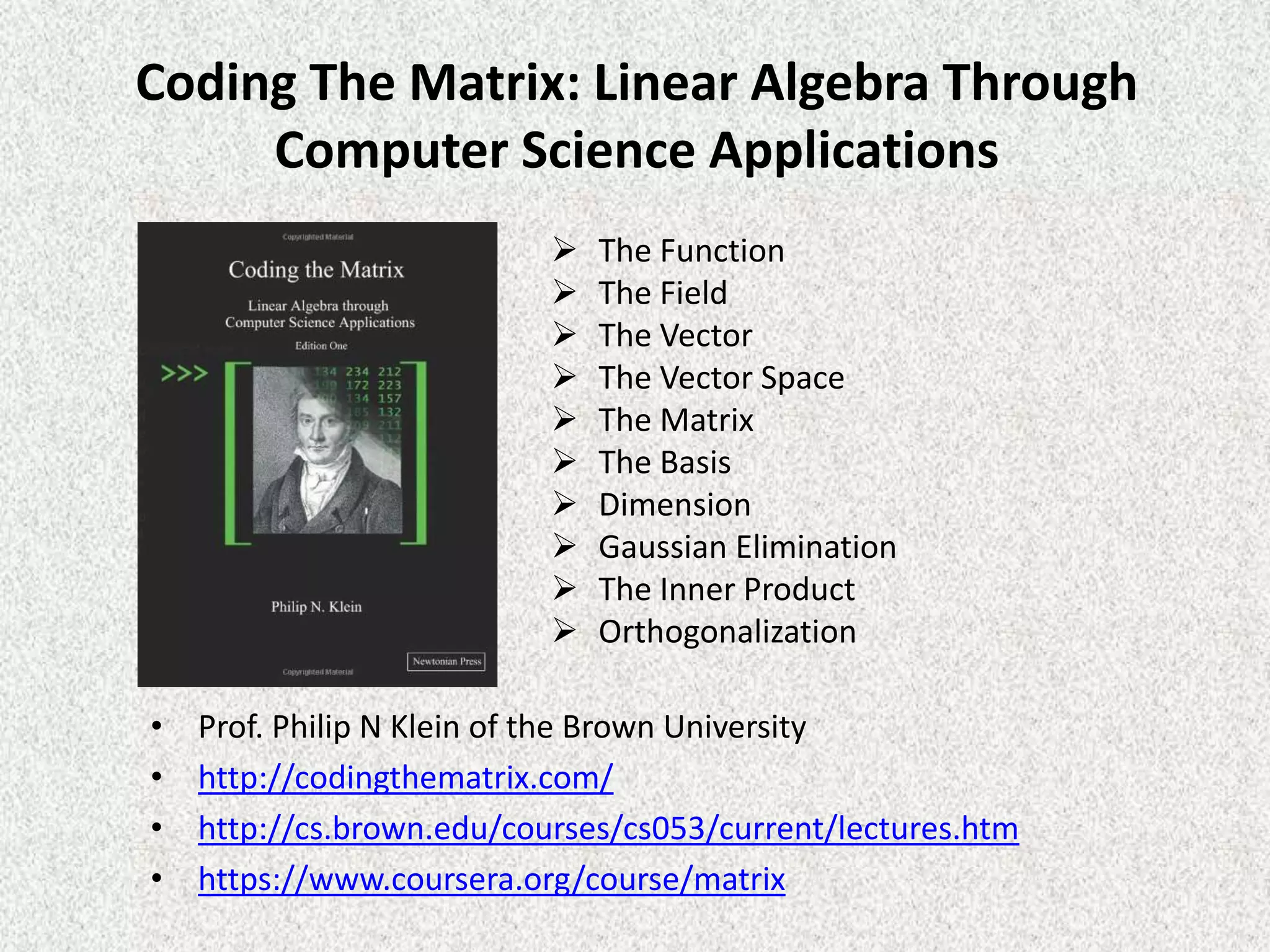
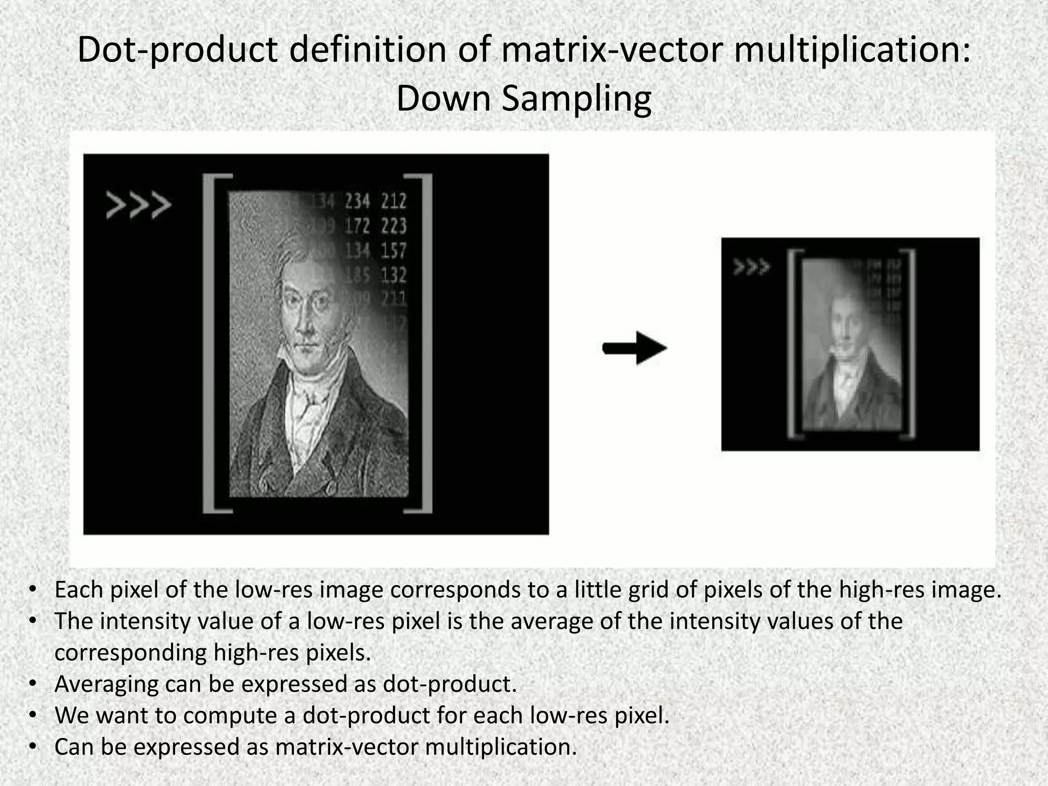
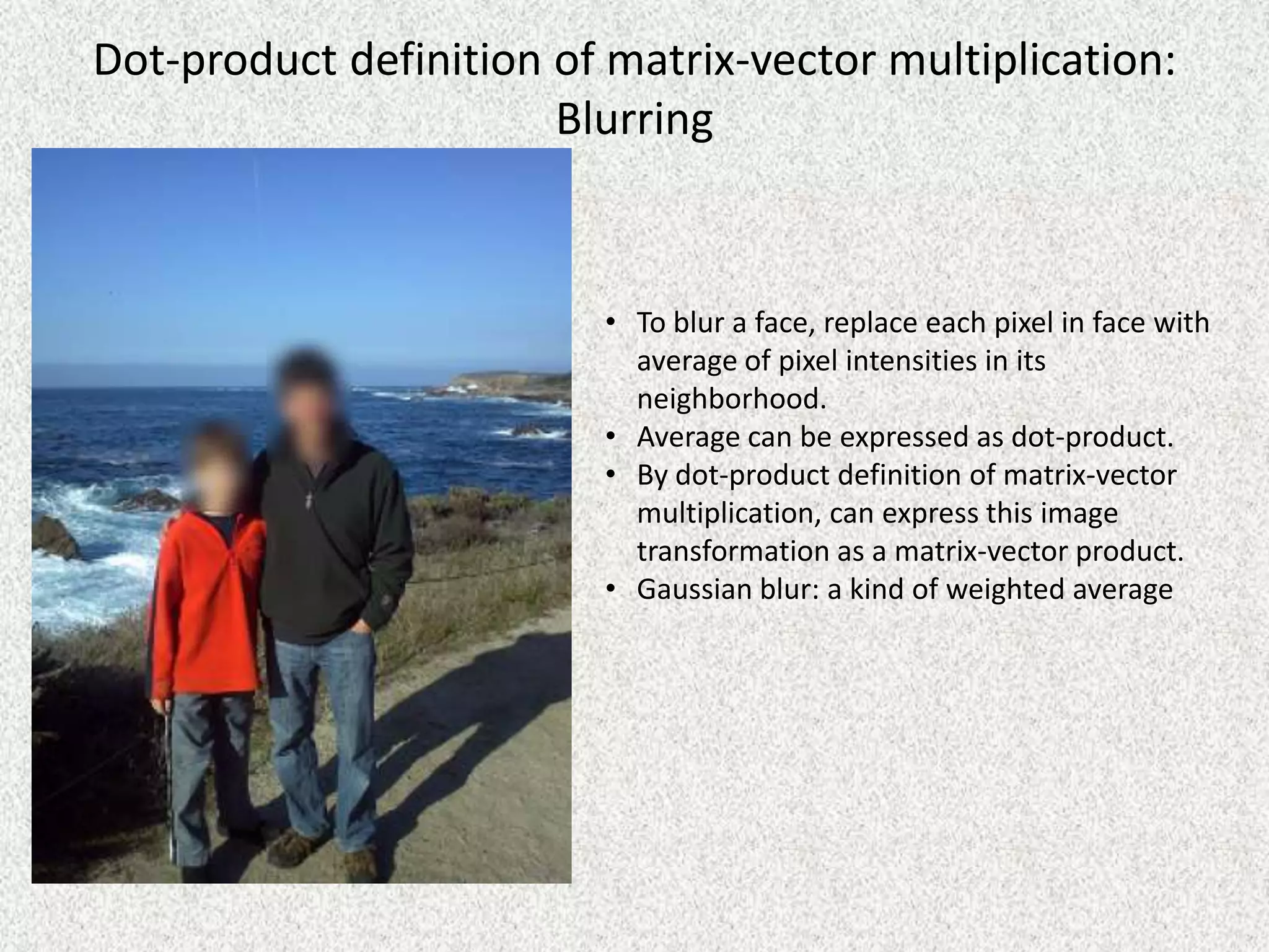
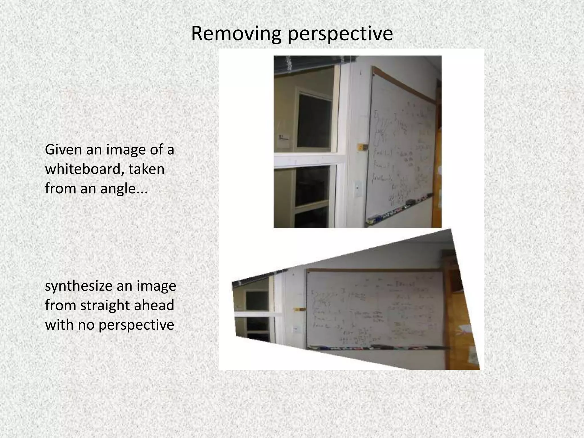
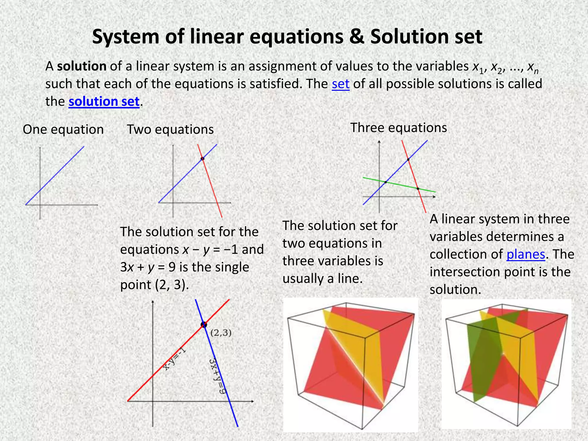
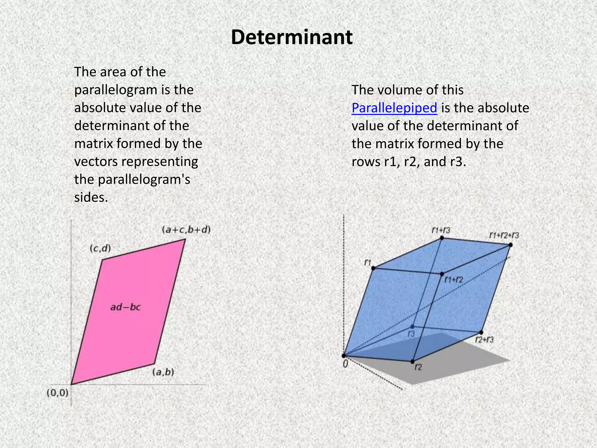
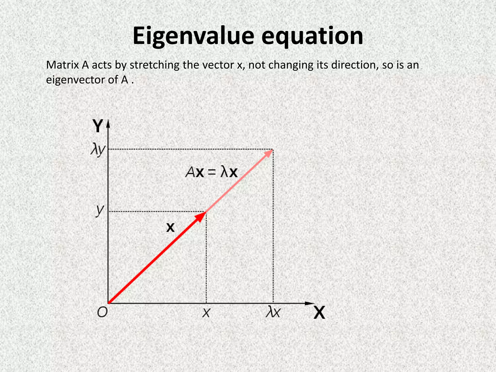
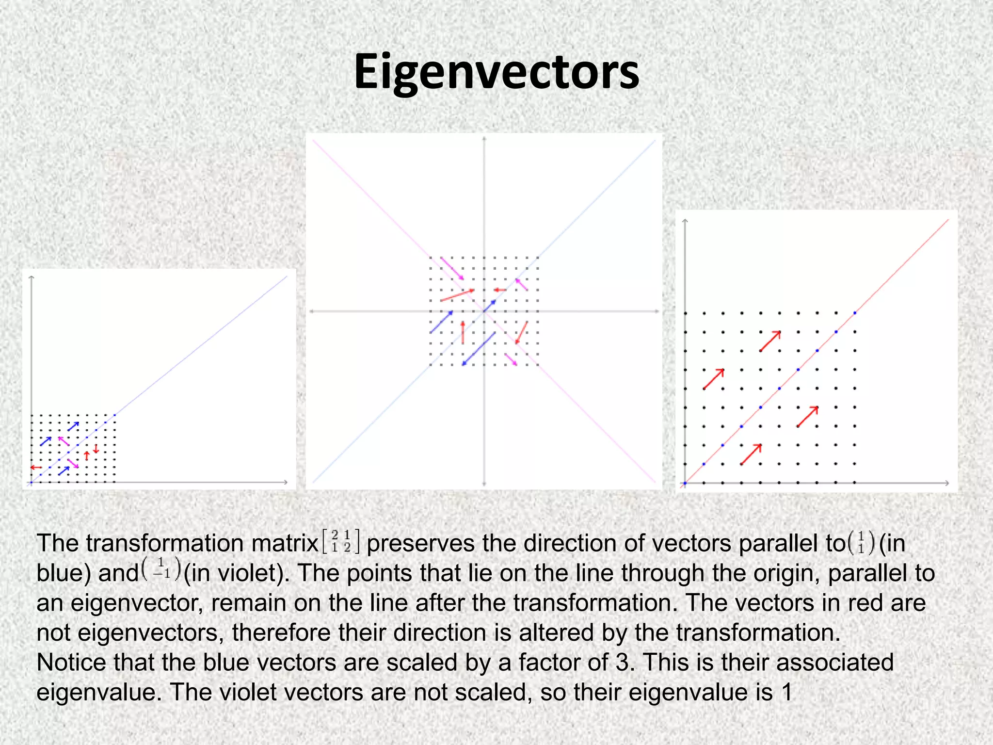
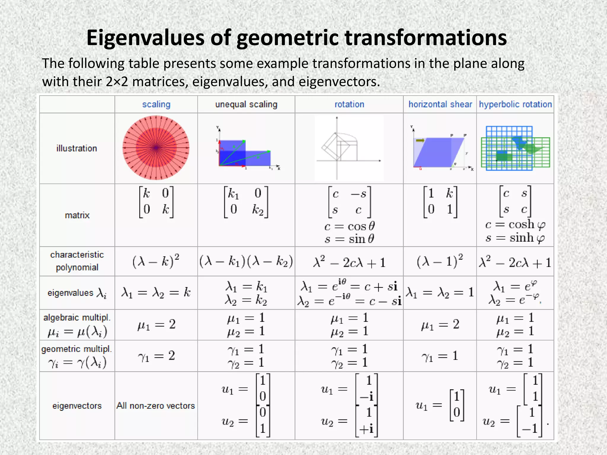
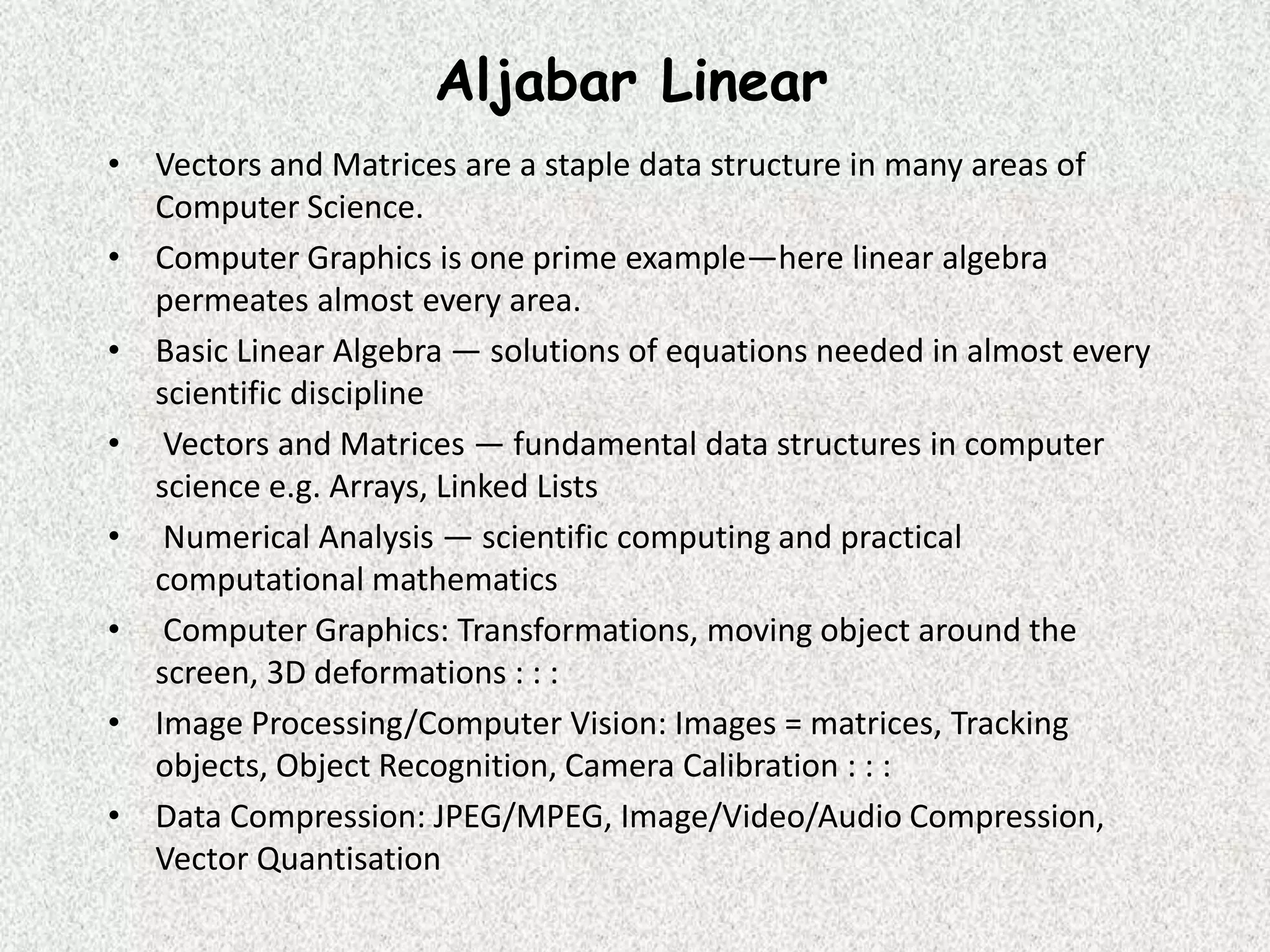
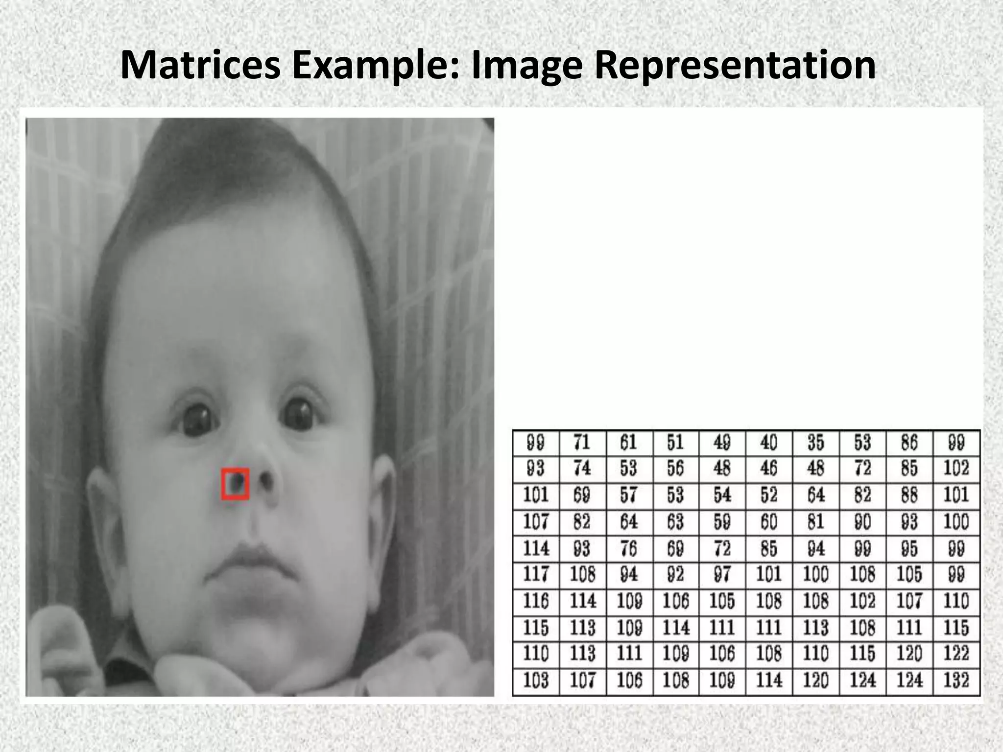
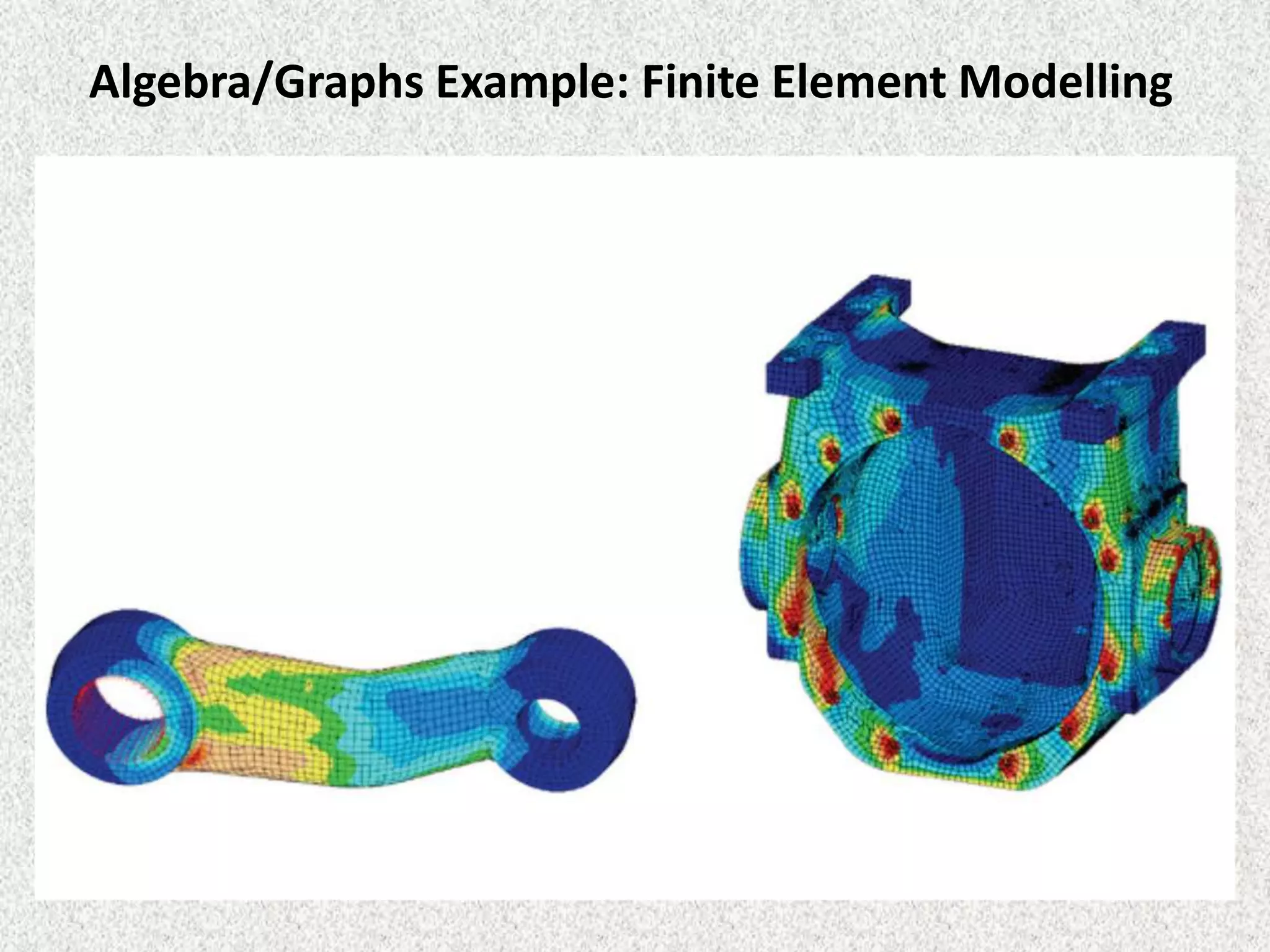
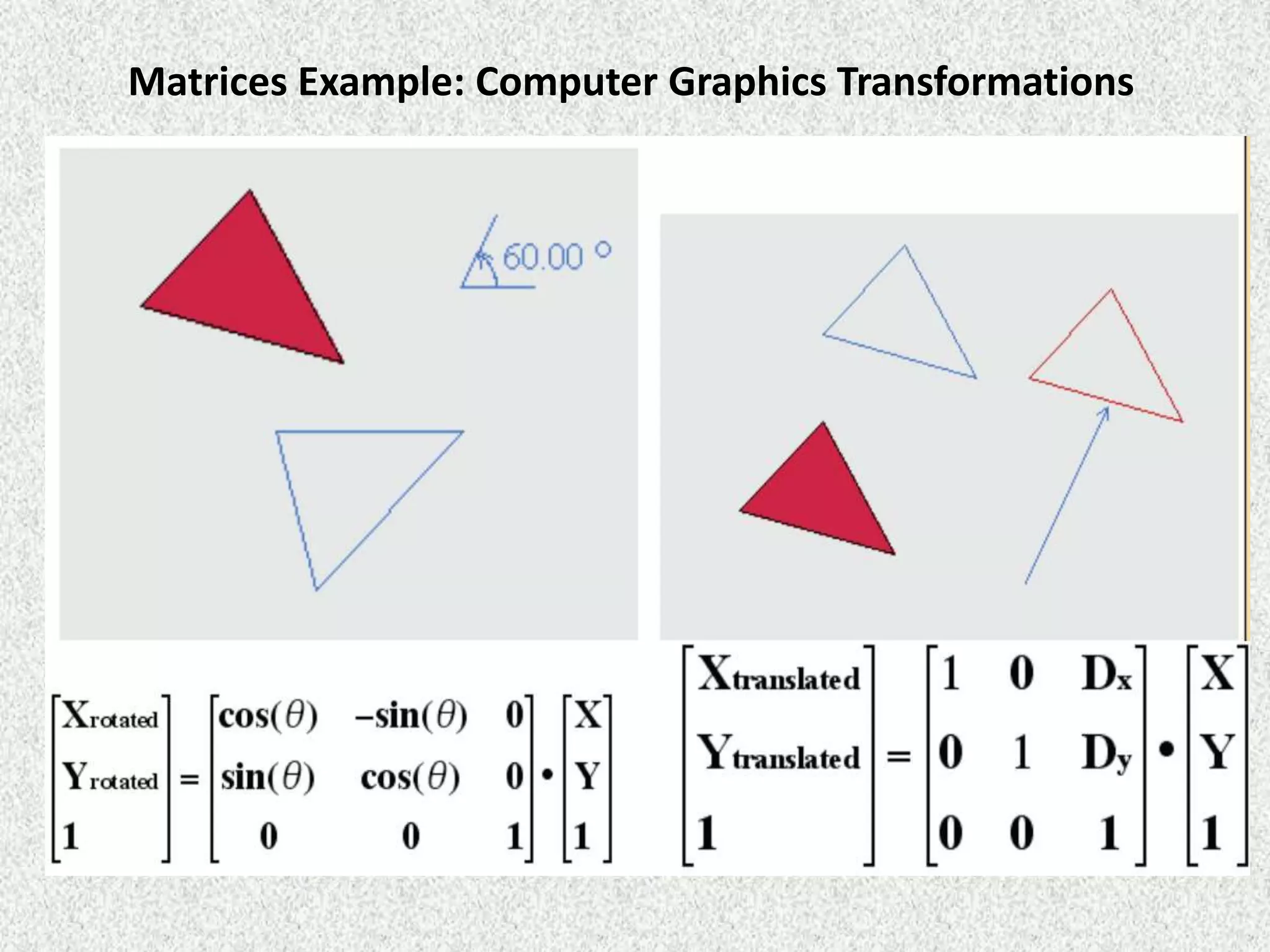
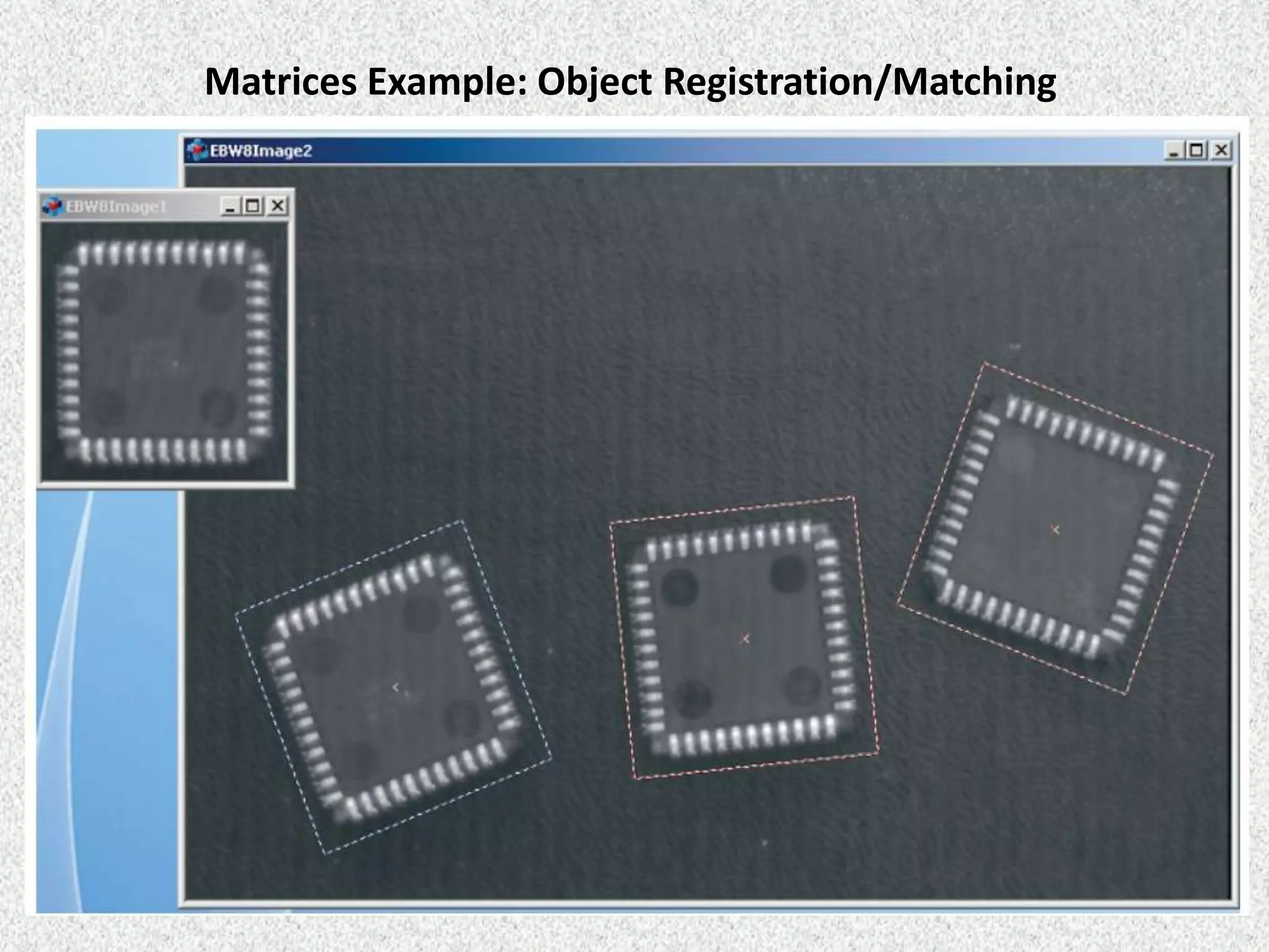
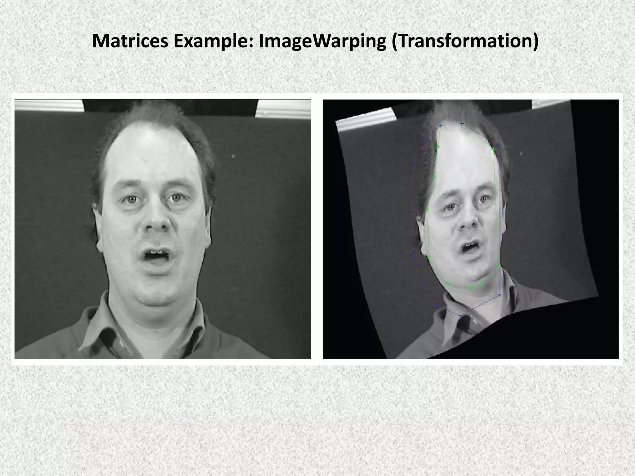
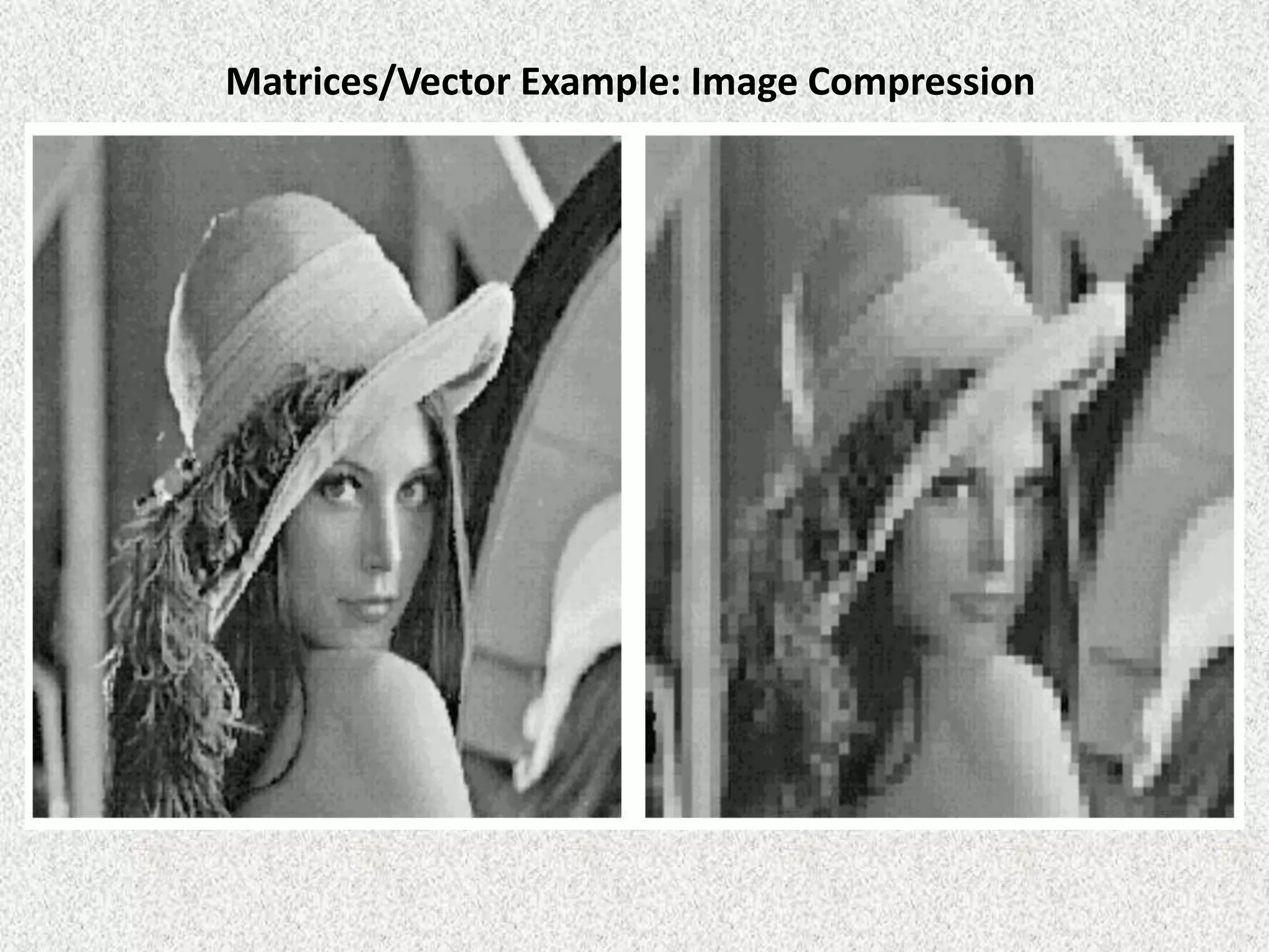
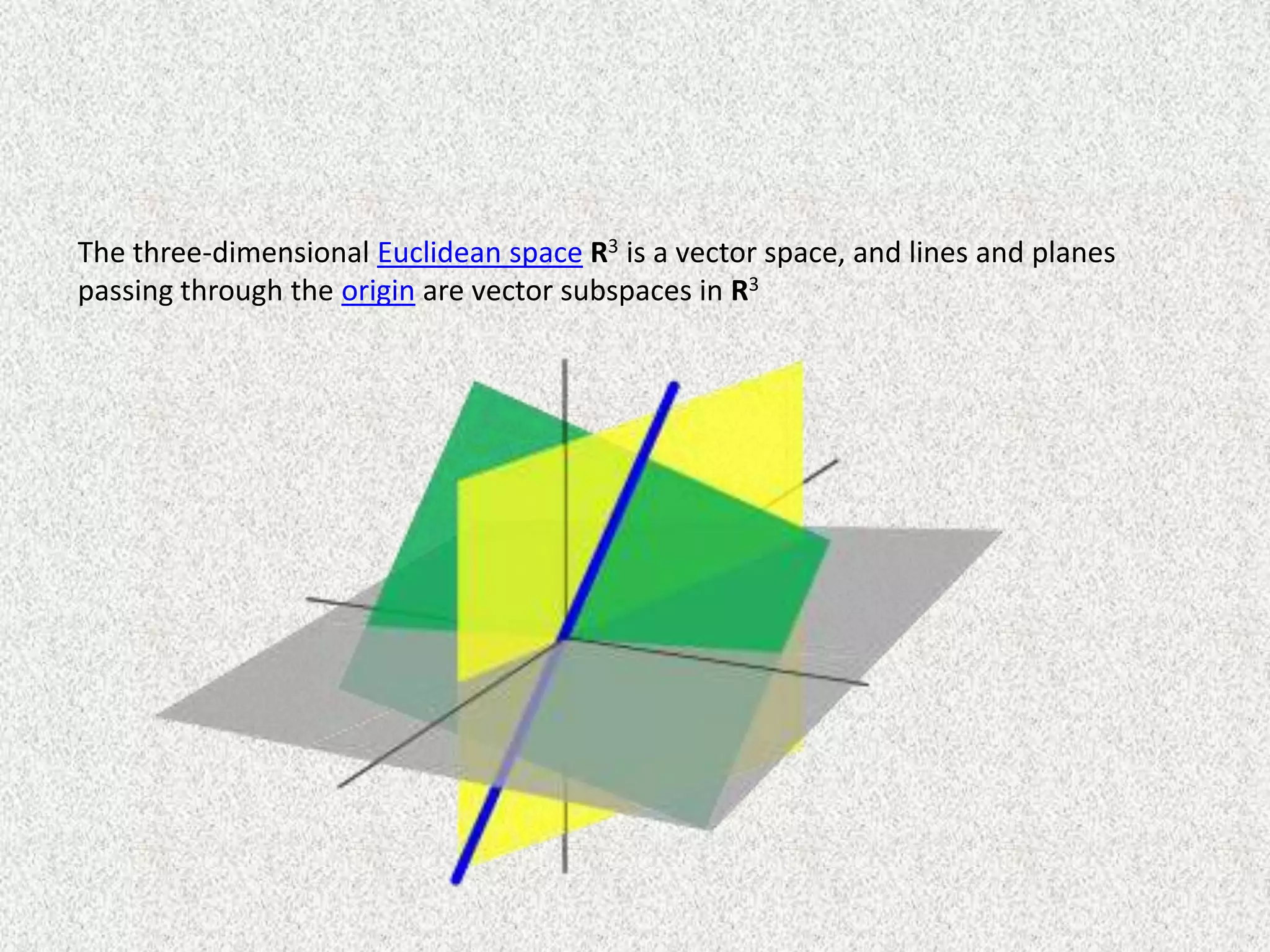
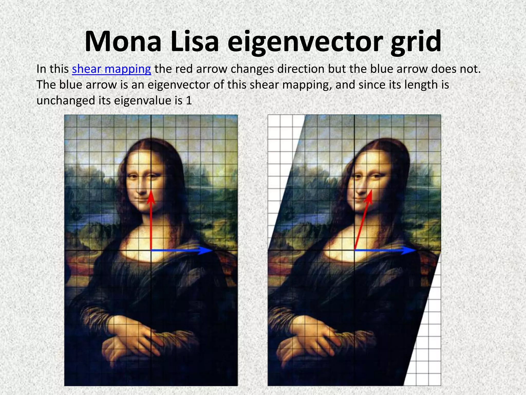
Kuliah Umum

Aljabar Linear
Rolly Rochmad Purnomo
rollyrp@yahoo.com

Universitas Serang Raya
11 Januari 2014
Aljabar Linear











System of Linear Equation & Matrices
Determinant
Vektor Ruang Dimensi 2 dan 3
Ruang Vektor Euclidean
General Vector Space
Inner Product Spaces
Eigen Value dan Eigen Vector
Linear Transformation
Applications
Computer Graphics
( Visualization of a Three-Dimensional Object)

Pi  Pj denotes that point Pi is connected to point Pj
Computer Graphics
( Visualization of a Three-Dimensional Object)
It should be noticed that only the x and y-coordinates of the vertices are needed by
the video display system to draw the view, because only the projection of the object
onto the xy-plane is displayed. However, we must keep track of the z-coordinates to
carry out certain transformations discussed later.
Computer Graphics
( Visualization of a Three-Dimensional Object)
We now show how to form new views of the object by scaling, translating, or
rotating the initial view. We first construct a 3 x n matrix P, referred to as the
coordinate matrix of the view, whose columns are the coordinates of the n points of
a view:
Computer Graphics
( Visualization of a Three-Dimensional Object)
Scaling
If a point Pi has coordinates
(Xi, Yi, Zi) in the original view, it is
to move to a new point Pi’ with
coordinates (Xi, Yi, Zi) in the
new view.

Pi’ = SPi

ex : scaled by =1, =0.5, =3
Computer Graphics
( Visualization of a Three-Dimensional Object)
Translation
to change an existing view so
that each point Pi with
coordinates (Xi, Yi, Zi) moves to a
new point Pi‘ with coordinates
(Xi+ Xo, Yi+ Yo, Zi+ Zo)

ex : scaled by Xo =1.2 , Yo =0.4, Zo =1.7
Computer Graphics
( Visualization of a Three-Dimensional Object)
Rotation  P’ = RP
rotated 90° about the x-axis
Computer Graphics
( Visualization of a Three-Dimensional Object)
Rotation  P’ = RP
rotated 90° about the y-axis
Computer Graphics
( Visualization of a Three-Dimensional Object)
Rotation  P’ = RP
rotated 90° about the z-axis
Computer Graphics
( Visualization of a Three-Dimensional Object)
Rotation  rotate first about the x-axis through 30°, then about the y-axis
through −70°, and finally about the z-axis through −27°  P’ = RP =R1R2R3P
CRYPTOGRAPHY: Hill Ciphers
A system of cryptography in which the plaintext is divided into sets of n letters, each of
which is replaced by a set of n cipher letters, is called a polygraphic system.
Hill ciphers is a class of polygraphic systems based on matrix transformations.
Example

Ciphertext vector = chipper x plaintext vector = Ap

Z=0
CRYPTOGRAPHY: Hill Ciphers
Z=0
Coding The Matrix: Linear Algebra Through
Computer Science Applications










•
•
•
•

The Function
The Field
The Vector
The Vector Space
The Matrix
The Basis
Dimension
Gaussian Elimination
The Inner Product
Orthogonalization

Prof. Philip N Klein of the Brown University
http://codingthematrix.com/
http://cs.brown.edu/courses/cs053/current/lectures.htm
https://www.coursera.org/course/matrix
Coding The Matrix
When you take a digital photo with your phone or
transform the image in Photoshop, when you play a video
game or watch a movie with digital effects, when you do a
web search or make a phone call, you are using
technologies that build upon linear algebra.
Linear algebra provides concepts that are crucial to many
areas of computer science, including graphics, image
processing, cryptography, machine learning, computer
vision, optimization, graph algorithms, quantum
computation, computational biology, information retrieval
and web search. Linear algebra in turn is built on two basic
elements, the matrix and the vector.
Combining vector addition and scalar multiplication
Vector addition = Translation (P’=P+T)
Scalar multiplication = Scaling (P’=SP) or rotating (P’=RP)
Example:
Combining vector addition and scalar multiplication
Matrix-Vector and Vector-Matrix Multiplication
Two ways to multiply a matrix by a vector:
• matrix-vector multiplication
• vector-matrix multiplication
For each of these, two equivalent definitions:

• in terms of linear combinations

• in terms of dot-products
Dot-product definition of matrix-vector multiplication:
Down Sampling

• Each pixel of the low-res image corresponds to a little grid of pixels of the high-res image.
• The intensity value of a low-res pixel is the average of the intensity values of the
corresponding high-res pixels.
• Averaging can be expressed as dot-product.
• We want to compute a dot-product for each low-res pixel.
• Can be expressed as matrix-vector multiplication.
Dot-product definition of matrix-vector multiplication:
Blurring

• To blur a face, replace each pixel in face with
average of pixel intensities in its
neighborhood.
• Average can be expressed as dot-product.
• By dot-product definition of matrix-vector
multiplication, can express this image
transformation as a matrix-vector product.
• Gaussian blur: a kind of weighted average
Removing perspective

Given an image of a
whiteboard, taken
from an angle...

synthesize an image
from straight ahead
with no perspective
Terima Kasih
System of linear equations & Solution set
A solution of a linear system is an assignment of values to the variables x1, x2, ..., xn
such that each of the equations is satisfied. The set of all possible solutions is called
the solution set.
One equation

Two equations

The solution set for the
equations x − y = −1 and
3x + y = 9 is the single
point (2, 3).

Three equations

The solution set for
two equations in
three variables is
usually a line.

A linear system in three
variables determines a
collection of planes. The
intersection point is the
solution.
Determinant
In linear algebra, the determinant is a value associated with a square matrix. It can
be computed from the entries of the matrix by a specific arithmetic
expression, while other ways to determine its value exist as well. The determinant
provides important information about a matrix of coefficients of a system of linear
equations, or about a matrix that corresponds to a linear transformation of a
vector space.
In the first case the system has a unique solution exactly when the determinant is
nonzero; when the determinant is zero there are either no solutions or many
solutions. In the second case the transformation has an inverse operation exactly
when the determinant is nonzero.
A geometric interpretation can be given to the value of the determinant of a
square matrix with real entries: the absolute value of the determinant gives the
scale factor by which area or volume (or a higher dimensional analogue) is
multiplied under the associated linear transformation, while its sign indicates
whether the transformation preserves orientation.
Thus a 2 × 2 matrix with determinant −2, when applied to a region of the plane
with finite area, will transform that region into one with twice the area, while
reversing its orientation.
Determinant
The area of the
parallelogram is the
absolute value of the
determinant of the
matrix formed by the
vectors representing
the parallelogram's
sides.

The volume of this
Parallelepiped is the absolute
value of the determinant of
the matrix formed by the
rows r1, r2, and r3.
Eigenvalue equation
Matrix A acts by stretching the vector x, not changing its direction, so is an
eigenvector of A .
Eigenvectors

The transformation matrix
preserves the direction of vectors parallel to (in
blue) and
(in violet). The points that lie on the line through the origin, parallel to
an eigenvector, remain on the line after the transformation. The vectors in red are
not eigenvectors, therefore their direction is altered by the transformation.
Notice that the blue vectors are scaled by a factor of 3. This is their associated
eigenvalue. The violet vectors are not scaled, so their eigenvalue is 1
Eigenvalues of geometric transformations
The following table presents some example transformations in the plane along
with their 2×2 matrices, eigenvalues, and eigenvectors.
Aljabar Linear
• Vectors and Matrices are a staple data structure in many areas of
Computer Science.
• Computer Graphics is one prime example—here linear algebra
permeates almost every area.
• Basic Linear Algebra — solutions of equations needed in almost every
scientific discipline
• Vectors and Matrices — fundamental data structures in computer
science e.g. Arrays, Linked Lists
• Numerical Analysis — scientific computing and practical
computational mathematics
• Computer Graphics: Transformations, moving object around the
screen, 3D deformations : : :
• Image Processing/Computer Vision: Images = matrices, Tracking
objects, Object Recognition, Camera Calibration : : :
• Data Compression: JPEG/MPEG, Image/Video/Audio Compression,
Vector Quantisation
Matrices Example: Image Representation
Algebra/Graphs Example: Finite Element Modelling
Matrices Example: Computer Graphics Transformations
Matrices Example: Object Registration/Matching
Matrices Example: ImageWarping (Transformation)
Matrices/Vector Example: Image Compression
The three-dimensional Euclidean space R3 is a vector space, and lines and planes
passing through the origin are vector subspaces in R3
Mona Lisa eigenvector grid
In this shear mapping the red arrow changes direction but the blue arrow does not.
The blue arrow is an eigenvector of this shear mapping, and since its length is
unchanged its eigenvalue is 1
Vibration analysis
Eigenvalue problems occur naturally in the vibration analysis of mechanical
structures with many degrees of freedom. The eigenvalues are used to determine
the natural frequencies (or eigenfrequencies) of vibration, and the eigenvectors
determine the shapes of these vibrational modes.
Cholesky decomposition
In linear algebra, the Cholesky decomposition or Cholesky factorization is a
decomposition of a Hermitian, positive-definite matrix into the product of a lower
triangular matrix and its conjugate transpose, useful for efficient numerical
solutions and Monte Carlo simulations. It was discovered by André-Louis Cholesky
for real matrices.
Cremer’s Rule
In linear algebra, Cramer's rule is an explicit
formula for the solution of a system of linear
equations with as many equations as unknowns,
valid whenever the system has a unique
solution. It expresses the solution in terms of
the determinants of the (square) coefficient
matrix and of matrices obtained from it by
replacing one column by the vector of right
hand sides of the equations. It is named after
Gabriel Cramer (1704–1752), who published the
rule for an arbitrary number of unknowns in
1750.

Geometric interpretation of Cramer's rule.
The areas of the second and third shaded
parallelograms are the same and the second
is X1 times the first. From this equality
Cramer's rule follows.

Kulum alin-11 jan2014

  • 1.
    Kuliah Umum Aljabar Linear RollyRochmad Purnomo rollyrp@yahoo.com Universitas Serang Raya 11 Januari 2014
  • 2.
    Aljabar Linear          System ofLinear Equation & Matrices Determinant Vektor Ruang Dimensi 2 dan 3 Ruang Vektor Euclidean General Vector Space Inner Product Spaces Eigen Value dan Eigen Vector Linear Transformation Applications
  • 3.
    Computer Graphics ( Visualizationof a Three-Dimensional Object) Pi  Pj denotes that point Pi is connected to point Pj
  • 4.
    Computer Graphics ( Visualizationof a Three-Dimensional Object) It should be noticed that only the x and y-coordinates of the vertices are needed by the video display system to draw the view, because only the projection of the object onto the xy-plane is displayed. However, we must keep track of the z-coordinates to carry out certain transformations discussed later.
  • 5.
    Computer Graphics ( Visualizationof a Three-Dimensional Object) We now show how to form new views of the object by scaling, translating, or rotating the initial view. We first construct a 3 x n matrix P, referred to as the coordinate matrix of the view, whose columns are the coordinates of the n points of a view:
  • 6.
    Computer Graphics ( Visualizationof a Three-Dimensional Object) Scaling If a point Pi has coordinates (Xi, Yi, Zi) in the original view, it is to move to a new point Pi’ with coordinates (Xi, Yi, Zi) in the new view. Pi’ = SPi ex : scaled by =1, =0.5, =3
  • 7.
    Computer Graphics ( Visualizationof a Three-Dimensional Object) Translation to change an existing view so that each point Pi with coordinates (Xi, Yi, Zi) moves to a new point Pi‘ with coordinates (Xi+ Xo, Yi+ Yo, Zi+ Zo) ex : scaled by Xo =1.2 , Yo =0.4, Zo =1.7
  • 8.
    Computer Graphics ( Visualizationof a Three-Dimensional Object) Rotation  P’ = RP rotated 90° about the x-axis
  • 9.
    Computer Graphics ( Visualizationof a Three-Dimensional Object) Rotation  P’ = RP rotated 90° about the y-axis
  • 10.
    Computer Graphics ( Visualizationof a Three-Dimensional Object) Rotation  P’ = RP rotated 90° about the z-axis
  • 11.
    Computer Graphics ( Visualizationof a Three-Dimensional Object) Rotation  rotate first about the x-axis through 30°, then about the y-axis through −70°, and finally about the z-axis through −27°  P’ = RP =R1R2R3P
  • 12.
    CRYPTOGRAPHY: Hill Ciphers Asystem of cryptography in which the plaintext is divided into sets of n letters, each of which is replaced by a set of n cipher letters, is called a polygraphic system. Hill ciphers is a class of polygraphic systems based on matrix transformations. Example Ciphertext vector = chipper x plaintext vector = Ap Z=0
  • 13.
  • 14.
    Coding The Matrix:Linear Algebra Through Computer Science Applications           • • • • The Function The Field The Vector The Vector Space The Matrix The Basis Dimension Gaussian Elimination The Inner Product Orthogonalization Prof. Philip N Klein of the Brown University http://codingthematrix.com/ http://cs.brown.edu/courses/cs053/current/lectures.htm https://www.coursera.org/course/matrix
  • 15.
    Coding The Matrix Whenyou take a digital photo with your phone or transform the image in Photoshop, when you play a video game or watch a movie with digital effects, when you do a web search or make a phone call, you are using technologies that build upon linear algebra. Linear algebra provides concepts that are crucial to many areas of computer science, including graphics, image processing, cryptography, machine learning, computer vision, optimization, graph algorithms, quantum computation, computational biology, information retrieval and web search. Linear algebra in turn is built on two basic elements, the matrix and the vector.
  • 16.
    Combining vector additionand scalar multiplication Vector addition = Translation (P’=P+T) Scalar multiplication = Scaling (P’=SP) or rotating (P’=RP) Example:
  • 17.
    Combining vector additionand scalar multiplication
  • 18.
    Matrix-Vector and Vector-MatrixMultiplication Two ways to multiply a matrix by a vector: • matrix-vector multiplication • vector-matrix multiplication For each of these, two equivalent definitions: • in terms of linear combinations • in terms of dot-products
  • 19.
    Dot-product definition ofmatrix-vector multiplication: Down Sampling • Each pixel of the low-res image corresponds to a little grid of pixels of the high-res image. • The intensity value of a low-res pixel is the average of the intensity values of the corresponding high-res pixels. • Averaging can be expressed as dot-product. • We want to compute a dot-product for each low-res pixel. • Can be expressed as matrix-vector multiplication.
  • 20.
    Dot-product definition ofmatrix-vector multiplication: Blurring • To blur a face, replace each pixel in face with average of pixel intensities in its neighborhood. • Average can be expressed as dot-product. • By dot-product definition of matrix-vector multiplication, can express this image transformation as a matrix-vector product. • Gaussian blur: a kind of weighted average
  • 21.
    Removing perspective Given animage of a whiteboard, taken from an angle... synthesize an image from straight ahead with no perspective
  • 22.
  • 23.
    System of linearequations & Solution set A solution of a linear system is an assignment of values to the variables x1, x2, ..., xn such that each of the equations is satisfied. The set of all possible solutions is called the solution set. One equation Two equations The solution set for the equations x − y = −1 and 3x + y = 9 is the single point (2, 3). Three equations The solution set for two equations in three variables is usually a line. A linear system in three variables determines a collection of planes. The intersection point is the solution.
  • 24.
    Determinant In linear algebra,the determinant is a value associated with a square matrix. It can be computed from the entries of the matrix by a specific arithmetic expression, while other ways to determine its value exist as well. The determinant provides important information about a matrix of coefficients of a system of linear equations, or about a matrix that corresponds to a linear transformation of a vector space. In the first case the system has a unique solution exactly when the determinant is nonzero; when the determinant is zero there are either no solutions or many solutions. In the second case the transformation has an inverse operation exactly when the determinant is nonzero. A geometric interpretation can be given to the value of the determinant of a square matrix with real entries: the absolute value of the determinant gives the scale factor by which area or volume (or a higher dimensional analogue) is multiplied under the associated linear transformation, while its sign indicates whether the transformation preserves orientation. Thus a 2 × 2 matrix with determinant −2, when applied to a region of the plane with finite area, will transform that region into one with twice the area, while reversing its orientation.
  • 25.
    Determinant The area ofthe parallelogram is the absolute value of the determinant of the matrix formed by the vectors representing the parallelogram's sides. The volume of this Parallelepiped is the absolute value of the determinant of the matrix formed by the rows r1, r2, and r3.
  • 26.
    Eigenvalue equation Matrix Aacts by stretching the vector x, not changing its direction, so is an eigenvector of A .
  • 27.
    Eigenvectors The transformation matrix preservesthe direction of vectors parallel to (in blue) and (in violet). The points that lie on the line through the origin, parallel to an eigenvector, remain on the line after the transformation. The vectors in red are not eigenvectors, therefore their direction is altered by the transformation. Notice that the blue vectors are scaled by a factor of 3. This is their associated eigenvalue. The violet vectors are not scaled, so their eigenvalue is 1
  • 28.
    Eigenvalues of geometrictransformations The following table presents some example transformations in the plane along with their 2×2 matrices, eigenvalues, and eigenvectors.
  • 29.
    Aljabar Linear • Vectorsand Matrices are a staple data structure in many areas of Computer Science. • Computer Graphics is one prime example—here linear algebra permeates almost every area. • Basic Linear Algebra — solutions of equations needed in almost every scientific discipline • Vectors and Matrices — fundamental data structures in computer science e.g. Arrays, Linked Lists • Numerical Analysis — scientific computing and practical computational mathematics • Computer Graphics: Transformations, moving object around the screen, 3D deformations : : : • Image Processing/Computer Vision: Images = matrices, Tracking objects, Object Recognition, Camera Calibration : : : • Data Compression: JPEG/MPEG, Image/Video/Audio Compression, Vector Quantisation
  • 30.
  • 31.
  • 32.
    Matrices Example: ComputerGraphics Transformations
  • 33.
    Matrices Example: ObjectRegistration/Matching
  • 34.
  • 35.
  • 36.
  • 37.
    The three-dimensional Euclideanspace R3 is a vector space, and lines and planes passing through the origin are vector subspaces in R3
  • 38.
    Mona Lisa eigenvectorgrid In this shear mapping the red arrow changes direction but the blue arrow does not. The blue arrow is an eigenvector of this shear mapping, and since its length is unchanged its eigenvalue is 1
  • 39.
    Vibration analysis Eigenvalue problemsoccur naturally in the vibration analysis of mechanical structures with many degrees of freedom. The eigenvalues are used to determine the natural frequencies (or eigenfrequencies) of vibration, and the eigenvectors determine the shapes of these vibrational modes.
  • 40.
    Cholesky decomposition In linearalgebra, the Cholesky decomposition or Cholesky factorization is a decomposition of a Hermitian, positive-definite matrix into the product of a lower triangular matrix and its conjugate transpose, useful for efficient numerical solutions and Monte Carlo simulations. It was discovered by André-Louis Cholesky for real matrices.
  • 41.
    Cremer’s Rule In linearalgebra, Cramer's rule is an explicit formula for the solution of a system of linear equations with as many equations as unknowns, valid whenever the system has a unique solution. It expresses the solution in terms of the determinants of the (square) coefficient matrix and of matrices obtained from it by replacing one column by the vector of right hand sides of the equations. It is named after Gabriel Cramer (1704–1752), who published the rule for an arbitrary number of unknowns in 1750. Geometric interpretation of Cramer's rule. The areas of the second and third shaded parallelograms are the same and the second is X1 times the first. From this equality Cramer's rule follows.