Downloaded 811 times

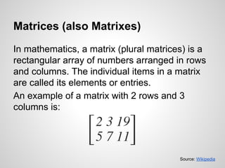
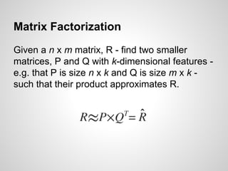
![Matrix Sparsity (or Density)
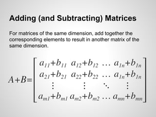
The percentage of non-zero elements to the
number of elements in total (and 1 - the ratio of
non-zero elements to the number of elements).
[ 11 22 0 0 0 0 0 ]
[ 0 33 44 0 0 0 0 ]
[ 0 0 55 66 77 0 0 ]
[ 0 0 0 0 0 88 0 ]
[ 0 0 0 0 0 0 99 ]](https://image.slidesharecdn.com/nonnegativematrixfactorization-140718204507-phpapp01/85/Beginners-Guide-to-Non-Negative-Matrix-Factorization-10-320.jpg)
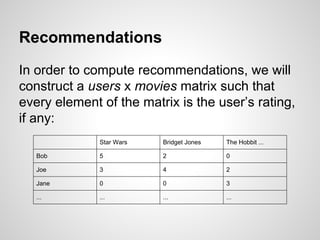

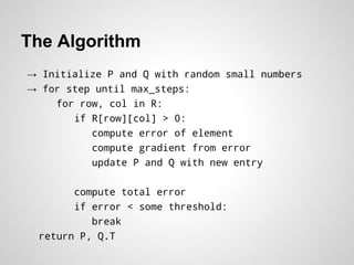
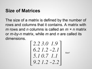
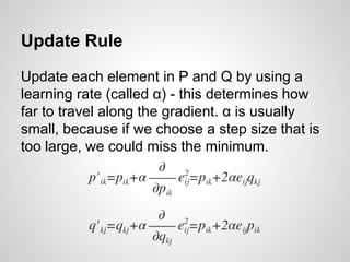
![The Algorithm
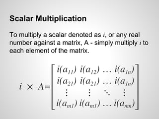
→ Initialize P and Q with random small numbers
→ for step until max_steps:
for row, col in R:
if R[row][col] > 0:
compute error of element
compute gradient from error
update P and Q with new entry
compute total error
if error < some threshold:
break
return P, Q.T](https://image.slidesharecdn.com/nonnegativematrixfactorization-140718204507-phpapp01/85/Beginners-Guide-to-Non-Negative-Matrix-Factorization-18-320.jpg)
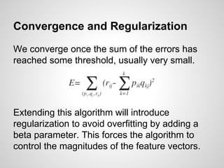
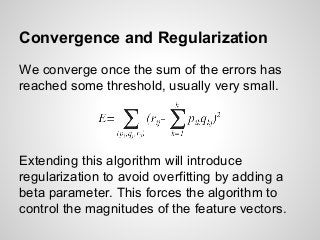
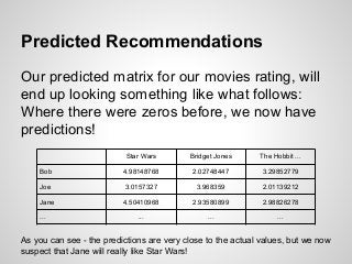

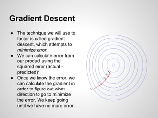
The document provides a tutorial on non-negative matrix factorization (NMF), explaining basic concepts of matrices, operations, and the factorization process. It describes how to approximate a given matrix using two smaller matrices and discusses applications in recommendation systems by filling in sparse matrices. The tutorial also outlines the algorithm, including gradient descent for minimizing error and regularization to avoid overfitting.


![Getting Started with Apache Spark: Big Data Made Simple [Free Meetup]](https://cdn.slidesharecdn.com/ss_thumbnails/apachesparkgettingstarted-260203175547-8361bcc3-thumbnail.jpg?width=640&height=640&fit=bounds)


