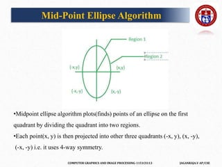
The document outlines a course on computer graphics and image processing, covering fundamental concepts, algorithms for drawing and transforming 2D and 3D graphics, and image processing techniques including raster and vector graphics. Key topics include line drawing algorithms such as the Digital Differential Analyzer (DDA) and Bresenham's algorithm, alongside practical applications and definitions related to computer graphics. Additionally, the course incorporates prerequisites and expected learning outcomes aligned with Bloom's taxonomy.


![COMPUTER GRAPHICS AND IMAGE PROCESSING-1151CS113 JAGANRAJA.V AP/CSE
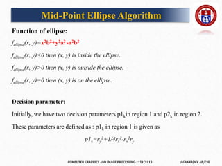
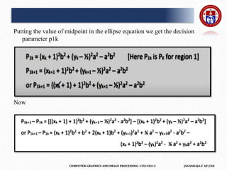
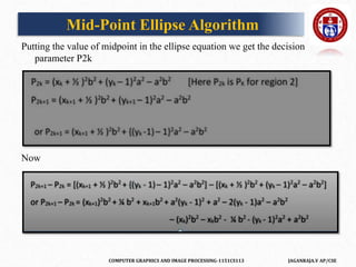
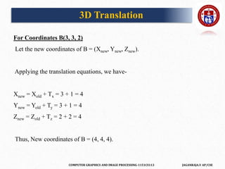
The Ellipse starts from (0,b), therefore putting (0,b) in P1k we get ,
P1k =(0+1)2b2+(b-1/2)2a2-a2b2
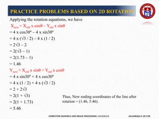
Or
P1k =b2+ b2 a2+1/4a2-a2b- a2b2
or
P1k =b2+1/4a2-a2b[initial decision parameter for first region]
Now, if P1k =>=0 then the next coordinate is (xk+1,yk-1)
Else if P1k <0 then the next coordinate is (xk+1,yk)
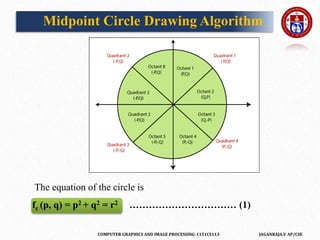
Mid-Point Ellipse Algorithm](https://image.slidesharecdn.com/tts2918cgipunit1-210302011431/85/COMPUTER-GRAPHICS-106-320.jpg)


![COMPUTER GRAPHICS AND IMAGE PROCESSING-1151CS113 JAGANRAJA.V AP/CSE
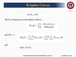
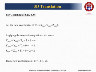
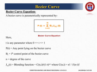
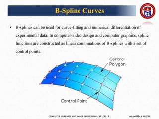
A B-spline curve is defined as a linear combination of control points Pi and B-
spline basis function Ni, k t given by
C(t)=∑ni=0PiNi,k(t), n≥k−1, tϵ[tk−1,tn+1]
Where,
• {pi: i=0, 1, 2….n} are the control points
• k is the order of the polynomial segments of the B-spline curve. Order k
means that the curve is made up of piecewise polynomial segments of
degree k - 1,
• the Ni,k(t) are the “normalized B-spline blending functions”. They are
described by the order k and by a non-decreasing sequence of real numbers
normally called the “knot sequence”.
B-Spline Curves](https://image.slidesharecdn.com/tts2918cgipunit1-210302011431/85/COMPUTER-GRAPHICS-274-320.jpg)