Download to read offline


![Matrices
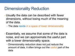
• An nm matrix A is a collection of n row vectors and m column
vectors
𝐴 =
| | |
𝑎1 𝑎2 𝑎3
| | |
𝐴 =
− 𝛼1
𝑇
−
− 𝛼2
𝑇
−
− 𝛼3
𝑇
−
• Matrix-vector multiplication
• Right multiplication 𝐴𝑢: projection of u onto the row vectors of 𝐴, or
projection of row vectors of 𝐴 onto 𝑢.
• Left-multiplication 𝑢𝑇
𝐴: projection of 𝑢 onto the column vectors of 𝐴, or
projection of column vectors of 𝐴 onto 𝑢
• Example:
1,2,3
1 0
0 1
0 0
= [1,2]](https://image.slidesharecdn.com/datamininglecture9-230924165916-d6802158/85/Data-Mining-Lecture_9-pptx-9-320.jpg)

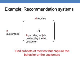
![Rank-1 matrices
• In a rank-1 matrix, all columns (or rows) are
multiples of the same column (or row) vector
𝐴 =
1 2 −1
2 4 −2
3 6 −3
• All rows are multiples of 𝑟 = [1,2, −1]
• All columns are multiples of 𝑐 = 1,2,3 𝑇
• External product: 𝑢𝑣𝑇 (𝑛1 , 1𝑚 → 𝑛𝑚)
• The resulting 𝑛𝑚 has rank 1: all rows (or columns) are
linearly dependent
• 𝐴 = 𝑟𝑐𝑇](https://image.slidesharecdn.com/datamininglecture9-230924165916-d6802158/85/Data-Mining-Lecture_9-pptx-11-320.jpg)

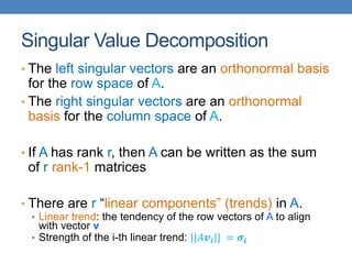
![Singular Value Decomposition
𝐴 = 𝑈 Σ 𝑉𝑇 = 𝑢1, 𝑢2, ⋯ , 𝑢𝑟
𝜎1
𝜎2
0
0
⋱
𝜎𝑟
𝑣1
𝑇
𝑣2
𝑇
⋮
𝑣𝑟
𝑇
• 𝜎1, ≥ 𝜎2 ≥ ⋯ ≥ 𝜎𝑟: singular values of matrix 𝐴 (also, the square roots
of eigenvalues of 𝐴𝐴𝑇 and 𝐴𝑇𝐴)
• 𝑢1, 𝑢2, … , 𝑢𝑟: left singular vectors of 𝐴 (also eigenvectors of 𝐴𝐴𝑇
)
• 𝑣1, 𝑣2, … , 𝑣𝑟: right singular vectors of 𝐴 (also, eigenvectors of 𝐴𝑇
𝐴)
𝐴 = 𝜎1𝑢1𝑣1
𝑇
+ 𝜎2𝑢2𝑣2
𝑇
+ ⋯ + 𝜎𝑟𝑢𝑟𝑣𝑟
𝑇
[n×r] [r×r] [r×m]
r: rank of matrix A
[n×m] =](https://image.slidesharecdn.com/datamininglecture9-230924165916-d6802158/85/Data-Mining-Lecture_9-pptx-13-320.jpg)


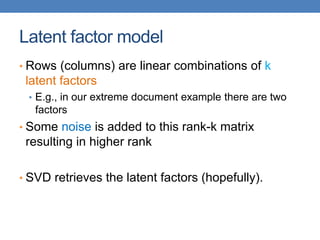

![Application: Recommender systems
• Data: Users rating movies
• Sparse and often noisy
• Assumption: There are k basic user profiles, and
each user is a linear combination of these profiles
• E.g., action, comedy, drama, romance
• Each user is a weighted cobination of these profiles
• The “true” matrix has rank k
• What we observe is a noisy, and incomplete version
of this matrix 𝐴
• The rank-k approximation 𝐴𝑘 is provably close to 𝐴𝑘
• Algorithm: compute 𝐴𝑘 and predict for user 𝑢 and
movie 𝑚, the value 𝐴𝑘[𝑚, 𝑢].
• Model-based collaborative filtering](https://image.slidesharecdn.com/datamininglecture9-230924165916-d6802158/85/Data-Mining-Lecture_9-pptx-23-320.jpg)


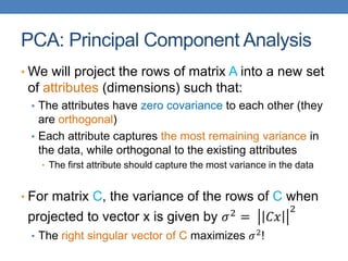

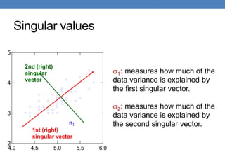


The document discusses dimensionality reduction techniques, specifically PCA and SVD, to address the challenges posed by high-dimensional data in data mining. It highlights the importance of reducing data dimensions while preserving essential information, using examples such as document matrices and recommendation systems. The text also covers linear algebra concepts relevant to these techniques, including eigenvectors, matrix decomposition, and applications like latent semantic indexing.