Some information on image intensities, eigenfaces and LDA--TODO

1. D
RA
FT
IMAGE PROCESSING, RETRIEVAL, AND ANALYSIS II: REPORT ON RESULTS
Raghunandan Palakodety
Universit¨at Bonn
Institut f¨ur Informatik
Bonn
ABSTRACT
This report presents the problem statements for three different
projects and illustrate the results that followed from practical
implementations in C++, using OpenCV framework. In im-
age processing and information theory, data compression is
found to be useful for transmitting or representing data with
relatively few number of bits. In the case of images, the prob-
ability distribution is not uniform and assigning equal number
of bits to each pixel can prove to be redundant. Now, im-
age quantization corresponds to reducing the number of bits
used for representing the image pixels at the expense of data
loss. This loss is not much noticeable. For this task, we used
iterative Lloyd-Max quantizer design which is non-uniform
quantizer. Dealing furthermore on image intensities, many
of face recognition pipelines include an image pre-processing
step. One such step is illumination compensation, employed
to cope with varying illumination. For addressing this prob-
lem, we used Retinex theory. The next project follows on
computing eigenfaces, an approach addressing high-level vi-
sual problem, face recognition. In this approach, we trans-
form face images into a small set of characteristic feature im-
ages known as eigenfaces, which are principal components of
the initial training set of images. Later, recognition is per-
formed by projecting a new image onto the subspace spanned
by eigenfaces. The final project includes two tasks. First task
being binary classification based on Fisher’s linear discrimi-
nant or LDA. Second task accentuates the merits of tensorial
discriminant classification, utilizes the concepts from tensor
algebra for the task of visual object recognition. This ap-
proach outperforms conventional LDA in terms of training
time and also addresses the singular scatter matrices, that is,
the small sample size problem.
Index Terms— image intensities, quantization, illumina-
tion correction, principal component analysis, linear discrim-
inant analysis, tensor contractions.
1. INTRODUCTION
This paper summarizes and highlights results of three projects
given. Problem specifications on image intensities, eigen-
faces and linear discriminant analysis were given and the im-
plementations were done using OpenCV framework, C++ and
QCustomplot. The outcomes of the given projects were
discussed to the best of our abilities, based on relevant ques-
tions that were posed.
The first project contains two tasks. First is implementation
of Llyod-Max algorithm for grey value quantization. Second
is estimating illumination plane parameters of an image that
corresponds to the best-fit plane from the image intensities.
The second project consists computing eigenfaces using a col-
lection of 2429 tiny face images of size 19x19. In this project,
we wish to find the principal components of the distribution
of faces and treating each image as a point in a very high di-
mensional space.
The third project focuses on object recognition and it con-
sists of two tasks. First is implementation of a binary clas-
sifier based on traditional Linear Discriminant Analysis or
LDA. Second task is tensor based Linear Discriminant Anal-
ysis which involves treating images as higher order tensors
instead of vectorizing the same. The theory behind this task
is taken from the paper [1] in which tensor contractions are
repeatedly applied to the given set of training examples and
uses alternating least squares to obtain an ρ term projection
tensor.
This paper is organized into sections in which the theoreti-
cal background of the project, the task specifications and out-
comes are discussed. This document ends with a conclusion
section, in which recent advents and improvements pertaining
to the projects are discussed.
2. THEORETICAL BACKGROUND FOR IMAGE
QUANTIZATION
This section describes image quantization and summarizes
the need for an algorithm or procedure to achieve end re-
sults. Quantization reduces ranges of values in a signal to
a single value. A quantizer maps the continuous variable
x into a discrete xq which takes values from a finite set
{r1, r2, r3, ...., rL} of numbers. The quantizer minimizes the
mean squared error for a given number of quantization levels
L. Let x, with 0 ≤ x ≤ A be a real scalar random variable
with a continuous probability density function (PDF) pX(x).
It is desired to find optimum boundaries or (decision) av and

2. D
RA
FT
the quantization (representation or reconstruction) points bv
for an L-level quantizer such that mean square error (MSE)
or quantization error E drops below a threshold or does not
improve significantly.
2.1. Llyod-Max quantization algorithm
For visualizing quantization curves, an intensity histogram
h(x) of a grey value image is converted into a density func-
tion p(x) using the following transformation,
p(x) =
h(x)
y h(y)
(1)
.
The following steps 1 and 2 describe the initialization of
boundaries and quantization points. Steps 3 and 4 are com-
puted iteratively [2].
1. Initialize the boundaries av of the quantization intervals
as
a0 = 0 (2)
av = v.
256
L
(3)
aL+1 = 256 (4)
2. Initialize the quantization or representation points bv as
follows
bv = v.
256
L
+
256
2.L
(5)
3. Iterate the following two steps
av =
bv + bv−1
2
(6)
4.
bv =
av+1
av
x.p(x).dx
av+1
av
p(x).dx
(7)
The above steps 3 and 4 are computed iteratively until the
quantization error drops below a threshold.
E =
L
v=1
av+1
av
(x − bv)2
.p(x).dx (8)
3. THEORETICAL BACKGROUND FOR
ILLUMINATION COMPENSATION
In image pre-processing algorithms it is necessary to com-
pensate for non-uniform lighting conditions. Illumination
conditions have an impact on facial features which attribute
towards robust face recognition. A study [3] performed by
NIST, on the progress made on face recognition under con-
trolled and uncontrolled illumination constraints, shows that
illumination has substantial effect on the recognition process.
The reason behind such illumination compensation proved to
be conducive for face recognition systems. Due to 3D shape
of human faces, a direct lighting source can produce strong
shadows that accentuate or diminish certain facial features.
In such a case, face recognition becomes arduous [4]. The
classic solution to this problem is applying histogram equal-
ization which produces optimal global contrast for a given
image. However, histogram equalization was considered as
a crude approach. Another approach proposed in [5] per-
forms logarithmic transformations to enhance low gray levels
and compress the higher ones. To recover an image under
assumed lighting condition, Quotient Image proposed in [6]
outperformed PCA.
Assuming reader is cognizant of lambertian surfaces, the
object surface’s irradiance is modeled using a mathemati-
cal equation, Quotient Image extracts the object’s surface
reflectance as an illumination invariant. More on model-
ing reflectance of opaque surfaces can be found BRDF (bi-
directional reflectance distribution function) theory.
The following approach is based on Retinex theory and
plane-subtraction or illumination gradient compensation al-
gorithm, which calculates a best-brightness plane to the im-
age under analysis and later subtracting this plane to the im-
age [4].
3.1. Illumination compensation
The reflectance model used in many cases can be expressed
as
I(x, y) = R(x, y).L(x, y) (9)
where I(x, y) is image pixel value, R(x, y) is the reflectance
and L(x, y) is the illumination at each point (x, y). The nature
of L(x, y) is determined by lighting source while R(x, y) is
determined by characteristics of the surface of object. There-
fore, R(x, y) which can be regarded as illumination insen-
sitive measure. Separating the reflectance R and the illumi-
nance L from real images is an ill-posed problem.
It is known from image pre-processing techniques that illu-
mination plane IP(x, y) of an image I(x, y) corresponds to
best-fit plane from the image intensities. IP(x, y) is a linear
approximation of I(x, y), given by
ansatz : IP(x, y) = ax + by + c (10)
Here, IP(x, y) is the intensity value of the pixel at loca-
tion (x, y)The above equation addresses 3-D regression plane
fitting problem [7]. The plane parameters a, b and c are esti-
mated by the linear regression formula as follows
p = (XT
X)−1
XT
x (11)
where p ∈ R3
is a vector that comprises the plane parameters
(a, b and c) and x ∈ Rn
is I(x, y) in a vector form where n is
the number of pixels. X ∈ Rnx3
is a matrix which holds the

3. D
RA
FT
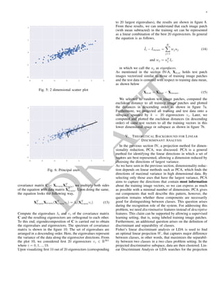
(a) (b)
Fig. 1. The image in (a) has an uneven illumination, while (b)
is the illumination compensated image.
(a) (b)
Fig. 2. The plot in (a) shows the image function f(x, y) with
x and y, while (b) image function f(x, y) along with illumi-
nation plane IP(x, y) and the contours.
pixels co-ordinates of the image under analysis. The first col-
umn contains the horizontal coordinates, the second column
the vertical coordinates and the entries in the third column are
set to value 1.
After estimating IP(x, y), this plane is subtracted from
I(x, y). This allows reducing shadows caused by extreme
lighting angles[4]. The results from our task on a set of two
input images are shown below. Figure 1 shows the same.
Another result of our experiment is shown in figure 3.
However, the changes are not conspicuous, but on perusal the
results show compensation. An additional step of Histogram
equalization can improve the results.
3-dimensional plot of the image function f(x, y) (shown in
figure 2a)along with the estimated illumination plane model
is shown in the figure 2b.
4. THEORETICAL BACKGROUND FOR
EIGENFACES AND PRINCIPAL COMPONENT
ANALYSIS
The eigenface approach for this classical pattern recognition
problem is to find the principal components of the distribu-
(a) (b)
Fig. 3. The image in (a) has an uneven illumination, while (b)
is illumination corrected image.
tion of the faces or the eigenvectors of the covariance matrix
of the set of face images, treating an image as in a very high
dimensional space. In this approach, we project training im-
age patches onto a lower-dimension space (sub-space) where
recognition is carried out. Since, we vectorize all the training
image patches before such a projection, each face image patch
I ∈ Rmxn
generates a huge dimensional input face space Rd
,
where d is m.n. Due to memory storage constraints and lim-
ited computational capacity, obtaining a parameterized model
in this high dimensional space is very difficult.
Dimensionality reduction of the input face space is the so-
lution and principal component analysis or PCA is one such
projection algorithm used, in order to obtain a reduced repre-
sentation of face images. Later in [8], these PCA projections
are used as feature vectors and similarity functions or distance
metrics such as Mahalobnis distance, Euclidean distance are
employed to to solve the problem of face recognition.
PCA was invented by Karl Pearson in 1901 and first published
in German as Karhunen-Lo`eve transformation or KLT[9], in
which a continuous transformation for de-correlating signals
was proposed. In this task, PCA is a powerful unsupervised
method for dimensionality reduction in data. It can be il-
lustrated using a two dimensional dataset. Consider the plot
shown in 5 for illustration of PCA. PCA finds the principal
axes in the data and explains the importance of those axes
that which describe the data distribution. Consider another
plot shown in figure 6, in which one of the vectors is no longer
than the other. This implies that data in the direction of longer
vector has significance greater than the data towards shorter
vector. After removing 5% of variance of this dataset and re-
projecting the data points on to the vector, the resulting plot
is shown in figure 4. The light shaded points are the original
data points and the dark blue points are the projected version.
This can be understood as dimensionality reduction.
Another approach for the task of face recognition is using
Fisher’s Linear discriminant analysis as projection algorithm
which will be dealt along with a novel and fast approach pro-
posed by [1].

4. D
RA
FT
Fig. 4. Approximating the dataset in lower dimension or di-
mensionality reduction
Fig. 5. 2 dimensional scatter plot
4.1. Computing eigenfaces
In this task we are given a collection of 2429 tiny face images
or image patches, each of size 19x19. From the given collec-
tion, we randomly chose 2186 as training images and rest 243
as test images. The images are read into a matrices X361x2186
train
and X361x243
test . The data matrix X361x2186
train is centered at zero
mean as
Xtrain = Xtrain − Xmean. (12)
The mean image computed is shown in the figure 9. Later,
the covariance matrix C. C = XtrainXT
train is computed in
a way that is conducive for eigenvalue decomposition. Note
that here covariance matrix is C361x361
. To compute the eigen
vectors of covariance matrix C = XtrainXT
train, we multiply
Fig. 6. Principal axes
both sides of the equation with data matrix XT
train. Upon do-
ing the same, the equation looks the following way,
XT
trainXtrain(XT
trainvi) = λi(XT
trainvi) (13)
Compute the eigenvalues λi and vi of the covariance matrix
C and the resulting eigenvectors are orthogonal to each other.
To this end, eigendecomposition of C is carried out to obtain
the eigenvalues and eigenvectors. The spectrum of covariance
matrix is shown in the figure 10. The set of eigenvalues are
arranged in a descending order. Here, the eigenvalues rep-
resent the variance of the data along the eigenvector direc-
tions. From the plot 10, we considered first 20 eigenvectors
vi ∈ R361
where i = 0, 1, .., 19.
Upon visualizing first 20 eigenvectors (corresponding to 20
largest eigenvalues), the results are shown in figure 8. From
these results, we can understand that each image patch (with
mean subtracted) in the training set can be represented as a
linear combination of the best 20 eigenvectors. In general the
equation is as follows,
ˆIi − Imean =
K
j=1
wjuj (14)
and wj = uT
j Ii.
in which we call the uj as eigenfaces.
As mentioned in the section 4.1, Xtest holds test patch images
vectorized similar to those of training image patches and the
test data is centered with respect to training data mean, as
shown below
Xtest = Xtest − Xmean. (15)
We selected 10 random test image patches, computed the
euclidean distance to all training image patches and plotted

5. D
RA
FT
(a)
(b)
Fig. 7. The plot in (a) shows distances of test image 0 to
all the training data while (b) displays the same except in a
lower-dimensional space.
the distances in descending order as shown in figure 7a. Fur-
thermore, we projected all training and test data onto a sub-
space spanned by k = 20 eigenvectors vi. Later, we com-
puted and plotted the euclidean distances (in descending or-
der) of same test vectors to all the training vectors in this
lower dimensional space or subspace as shown in figure 7b.
5. THEORETICAL BACKGROUND FOR LINEAR
DISCRIMINANT ANALYSIS
In the previous section 4, a projection method for dimension-
ality reduction, PCA, was discussed. PCA is a general method
for identifying the linear directions in which a set of vectors
(a) (b) (c) (d) (e) (f) (g) (h) (i) (j)
(k) (l) (m) (n) (o) (p) (q) (r) (s) (t)
Fig. 8. Visualizing 20 eigen vectors
Fig. 9. Mean image computed from training samples.
Fig. 10. Spectrum of covariance
are best represented, allowing a dimension reduced by choos-
ing the directions of largest variance.
As we have seen in the previous section, dimensionality re-
duction depends on linear methods such as PCA, which finds
the directions of maximal variance in high dimensional data.
By selecting only those axes that have the largest variance,
PCA aims to capture the directions that contain most infor-
mation about the training image vectors, so we can express as
much as possible with a minimal number of dimensions. PCA
gives out components that well describe this pattern, however,
the question remains whether those components are necessar-
ily good for distinguishing between classes. This question
arises during the recognition role of the system. For address-
ing this problem, we need discriminative features instead of
descriptive features. This claim can be supported by allowing
a supervised learning setting, that is, using labeled training
image patches. Furthermore, an additional question arises on
the definition of discriminant and separability of classes.
Fisher’s linear discriminant analysis or LDA is used to find an
optimal linear projection W, that captures major difference
between classes, in other words, that maximizes the separa-
bility between two classes in a two class problem setting. In
the projected discriminative subspace, data are then clustered
[10]. Linear Discriminant Analysis or LDA searches for the
projection axes on which the input vectors of two different
classes are far away from each other and at the same time in-
put vectors of same class are close to each other [10]. Among
all such infinitely many projection axes or lines, a line is cho-
sen that maximally separates the projected data [11]. The
solution to this problem is obtained by solving the general
eigensystem of within-class and between-class scatter matri-
ces.

6. D
RA
FT
LDA for binary classification requires supervised setting. A
collection of n labeled training data
{(xi, yi)}n
i=1 (16)
where the data vectors xi ∈ Rm
are from two classes C1
and C2 and the labels yi ∈ {+1, −1} indicate class member-
ship in such way,
yi =
+1, if xi ∈ C1
−1, if xi ∈ C2
the task requires us to determine a classifier y(x) that assigns
or predicts an unknown/unseen or new data point, a class la-
bel [11].
One way to view a linear classification model is in terms
of dimensionality reduction. Consider first the case of two
classes, and suppose we take m dimensional input vector xi
and project it down to one dimension using
y = wT
x (17)
If we place a threshold on y and classify y ≥ −w0 as class C1
and otherwise class C2. In general, the projection onto one
dimension leads to a considerable loss of information, and
classes that are well separated in the original m dimensional
space may become strongly overlapping in one dimension.
The simplest measure of separation of the classes when pro-
jected onto w is the separation of the projected class means.
The problem boils down to choosing w so as to maximize
m2 − m1 = wT
(m2 − m1) (18)
where,
mk = wT
mk (19)
is the mean of the projected images from class Ck. The pro-
jection formula shown in (17) transforms the set of labeled
data points in x into a labeled set in the one-dimensional space
y. The within-class variance of the transformed data from
class Ck is given by
s2
k =
n∈Ck
(yn − mk)2
(20)
where yn = wT
xn. From [11] we can derive total within
class-variance for the whole dataset to be simply s2
1 + s2
2 as
shown below
s2
k =
n∈Ck
(yn − mk)2
=
n∈Ck
(wT
x − wT
mk)2
=
n∈Ck
wT
(x − mk)(x − mk)T
w
= wT
Skw
(21)
Now using equation (21), in the process of yielding
Raleigh co-efficient, rewrite within-class scatter matrix as,
SW = S1 + S2 (22)
s2
1 + s2
2 = wT
S1w + wT
S2w
= wT
SW w
(23)
Following [11], we want the distance between the pro-
jected means m1 and m2 to be as large as possible.
| m1 − m2 |2
=| wT
m1 − wT
m2 |2
(24)
where projected means m1 and m2 are as shown in equa-
tion (25).
m1 =
1
N1
x∈C1
wT
x
m2 =
1
N2
x∈C2
wT
x
(25)
The equation in (24) can be written as,
| m1 − m2 |2
=| wT
m1 − wT
m2 |2
= wT
(m1 − m2)(m1 − m2)T
w
= wT
SBw
(26)
Following [11], Fisher’s linear discriminant is defined
as the linear function wT
x that maximizes the following ob-
jective/distortion function J(w),
J(w) =
(m1 − m2)2
s2
1 + s2
2
(27)
Substituting (23), (24) in (27) and we need to find an op-
timal w∗
, that maximizes (27) and must satisfy
SBw = λSW w (28)
From [11], optimal projection is,
w∗
= S−1
W (m1 − m2) (29)
The intuition behind the equation (29) is projecting the
data on to one dimension that maximizes the ratio of between-
class scatter and total within-class scatter.
The first task of this project measures the performance lin-
ear discriminant analysis or LDA for the case of binary clas-
sification. The second task of this project uses tensors [12] of
rank 2 as training vectors (instead of vectorizing the training
images) for the same task of binary classification.

7. D
RA
FT
5.1. Applying Fisher’s linear discriminant analysis: Ex-
perimental setting
A collection of 2556 training image patches of which 2442
are patches of background, tagged as class label C2, whereas
the rest 124 are patches of containing cars and tagged as class
label C1. Each of these ground truth image patches is of size
81 × 31. The 2D visualization of projection vector w com-
puted is shown in figure 11. From this figure, which is ob-
tained from least squares regression training, there is no car-
like structural traits upon visualization of w.
Fig. 11. 2D visualization of projection vector
w = (XT
X)−1
XT
y
5.2. Applying classifier on test data
We used k = 1, 2, ...10 different classifiers as shown below
y(x) =
+1, if wT
x ≥ θk
−1, otherwise
where θk ∈ [µ1, µ2]. µ1 and µ2 are projected means.
Before applying the best performing classifier on test set
of 170 images, we plotted the precision-recall curve on the
training set. Precision and recall often show an inverse rela-
tionship, that is, increasing one goes along with the cost of
reducing the other. Applying the best performing classifier
(among the 10 classifiers), the figure 12 shows results on an
image with single target (car).
6. THEORETICAL BACKGROUND FOR TENSOR
LINEAR DISCRIMINANT ANALYSIS
In the previous approach discussed in section 5, where train-
ing image patches x ∈ Rm×n
of size m × n are vectorized
(a) (b)
Fig. 12. The figure in (a) and (b) shows a car bounded by a
rectangle upon applying the classifier with threshold.
(a) (b) (c)
Fig. 13. W =
ρ
r=1 urvT
r
into mn, instead, treating images for what they are, we use
tensors [1]. In the procedure proposed in [1], we compute
the projection tensor by applying tensor contractions to the
given set of training image patches and use alternating least
squares.
A tensor also known as n-way array or multidimensional
matrix or n-mode matrix, is a higher order generalization
of a vector (first order tensor) and a matrix (second order
tensor). In this short description on second order tensors
X ∈ Rm×n
, we use calligraphic upper-case letters X ,
to represent grey-value images of size m × n. A train-
ing set {(X α
, yα
)}α=1,2,...N of N image patches, where
X α
∈ Rm×n
is given. Tensor discriminant analysis re-
quires a projection tensor W which solves the regression
problem[1],
W = arg min
W∗
α
(yα
− W∗
X α
)2
(30)
6.1. Applying tensor discriminant analysis: Experimen-
tal setting
As described in section 5.1, we use the same image collection
for training and test data. We determine a projector W where,
W =
ρ
r=1
urvT
r (31)
A random initialization of u, we compute a set of vectors
xα
from tensor contractions X α
kluk and inserting them into
a design matrix X and use equation w = (XT
X)−1
XT
y to
compute v. Now, having v, we compute for u and iteratively
until the error converges ur(t) − ur(t − 1) ≤ . Follow-
ing the algorithm [1] for computing a second order tensor
discriminant classifier W, we compute ρ-term solution of
second order projection tensor as W = r ur ⊗ vr.
Visualizing the ρ-term solution of second order projection
tensors, we observe (shown in figure 13) car-like structural
traits which was not in the case of conventional linear dis-
criminant analysis [1]. The figures for (a)ρ = 1, (b)ρ = 3 and
(c)ρ = 9 show the projection tensors respectively.
The mutlilinear classifier maps the training samples onto
the best discriminant direction, the results of the implemen-
tation proposed in [1] are shown in the figures 14a, 14b and
14c. In figure 14c, an overlap is observed.
While implementation, the training time of this approach no-
ticeably outperforms the conventional LDA (running time is

8. D
RA
FT
(a) (b) (c)
Fig. 14. Projections produced by the tensor predictor
not reported). Adding to the list of advantages is that this
approach addresses the problem of singular matrices (which
is often in the case where dimensionality of input space is
greater than the number of samples).
7. CONCLUSION
In discriminant analysis, linear discriminant analysis com-
putes a transformation that maximizes the between-class scat-
ter while minimizing the within-class scatter. Such a trans-
formation must retain the class separability while reducing
the variation due to sources other than illumination. While
conventional LDA takes huge running time for training the
projector, tensorial based approach outperforms the former in
this aspect. Also to alleviate the small sample size problem,
we can perform two projections. PCA can be applied to the
data set to reduce its dimensionality and LDA is then applied
further reduce the dimensionality. However, the major advan-
tage of tensor discriminant classifiers is that rank deficiency
constraint considerably reduces the number of free parame-
ters which makes the multi-linear classifiers faster and pre-
ferred.
In the case of linear methods for dimensionality reduction and
unsupervised techniques, in PCA, there are limitations on the
kinds of feature dimensions that can be extracted. For many
generalized object detection problems, the features that mat-
ter are not easy to express. It becomes really difficult to select
those features where the algorithm needs to classify apart cats,
from faces, from cars. We need to extract information rich di-
mensions from our input images.
Autoencoders overcome these limitations by exploiting the in-
herent non-linearity of neural networks. An autoencoder [13]
comes under the category of unsupervised learning that uti-
lizes a neural network to produce a low-dimensional repre-
sentation of a high-dimensional input. It consists of two ma-
jor parts, the encoder and the decoder networks, in which, the
former is used during both training and testing, latter being
used only during training.
8. REFERENCES
[1] C. Bauckhage and T. Kaster, “Benefits of separa-
ble, multilinear discriminant classification,” in Pattern
Recognition, 2006. ICPR 2006. 18th International Con-
ference on, Aug 2006, vol. 4, pp. 959–959.
[2] Prof. Christian Bauckhage, “Image processing,retrieval,
and analysis (ii),” [online], 2015, https://sites.
google.com/site/bitimageprocessing/
home/lecture-notes-ii.
[3] P Jonathon Phillips, W Todd Scruggs, Alice J OToole,
Patrick J Flynn, Kevin W Bowyer, Cathy L Schott, and
Matthew Sharpe, “Frvt 2006 and ice 2006 large-scale
results,” 2007.
[4] Javier Ruiz-del Solar and Julio Quinteros, “Illumi-
nation compensation and normalization in eigenspace-
based face recognition: A comparative study of different
pre-processing approaches,” Pattern Recognition Let-
ters, vol. 29, no. 14, pp. 1966–1979, 2008.
[5] Hong Liu, Wen Gao, Jun Miao, Debin Zhao, Gang
Deng, and Jintao Li, “Illumination compensation and
feedback of illumination feature in face detection,” in
Info-tech and Info-net, 2001. Proceedings. ICII 2001
- Beijing. 2001 International Conferences on, 2001,
vol. 3, pp. 444–449 vol.3.
[6] Amnon Shashua and Tammy Riklin-Raviv, “The quo-
tient image: Class-based re-rendering and recognition
with varying illuminations,” IEEE Trans. Pattern Anal.
Mach. Intell., vol. 23, no. 2, pp. 129–139, Feb. 2001.
[7] Prof. Christian Bauckhage, “Image processing,retrieval,
and analysis (ii),” [online], 2015, https://sites.
google.com/site/bitimageprocessing/
home/lecture-notes-ii.
[8] Matthew Turk, Alex P Pentland, et al., “Face recogni-
tion using eigenfaces,” in Computer Vision and Pattern
Recognition, 1991. Proceedings CVPR’91., IEEE Com-
puter Society Conference on. IEEE, 1991, pp. 586–591.
[9] K. Karhunen, Ueber lineare Methoden in der
Wahrscheinlichkeitsrechnung, Annales Academiae sci-
entiarum Fennicae. Series A. 1, Mathematica-physica.
1947.
[10] Ying Wu, “Principal component analysis and lin-
ear discriminant analysis,” Electrical Engineering and
Computer Science, Northwestern University, Evanston,
wykład, 2014.
[11] Prof. Christian Bauckhage, “Image processing,retrieval,
and analysis (ii),” [online], 2015, https://sites.
google.com/site/bitimageprocessing/
home/lecture-notes-ii.
[12] Prof. Christian Bauckhage, “Image processing,retrieval,
and analysis (ii),” [online], 2015, https://sites.
google.com/site/bitimageprocessing/
home/lecture-notes-ii.

9. D
RA
FT
[13] Yoshua Bengio, “Learning deep architectures for ai,”
Foundations and Trends in Machine Learning, vol. 2,
no. 1, pp. 1–127, 2009.