
Recommended
Recommended
More Related Content
Similar to nonlinear.pptx
Similar to nonlinear.pptx (20)
Recently uploaded
Recently uploaded (20)
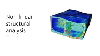
nonlinear.pptx
- 2. Introduction • The FEM is the most powerful tool for solving constitutive equations over complicated systems • An advantage of the FEM based modeling is that it enables the consideration of complex geometries and may attribute different material properties to various components of a system • since the 1970s, many commercial finite element software companies have evolved: ANSYS, ABAQUS, COMSOL, ADINA, LS-DYNA, and MARC • The Definition of material model is any product will deform when exposed to a load • The presentation is composed of seven main parts
- 3. Part 1 Difference between liner and non-liner analysis Liner analysis • linear relationship between the applied loads and the response of the system. • This means that in a linear analysis the flexibility of the structure need only be calculated once (by assembling the stiffness matrix and inverting it). • This principle of superposition of load cases assumes that the same boundary conditions are used for all the load cases. Nonlinear analysis • the structure's stiffness changes as it deforms. • a nonlinear relation holds between applied forces and displacements • All physical structures exhibit nonlinear behavior • Nonlinear effects can originate from geometrical nonlinearity’s • Modern analysis software makes it possible to obtain solutions to nonlinear problems. The difference between linear and non-linear analyses applied on a structure depends on several parameters, such as: - Mechanical behavior of the structure (it depends on the construction material); - Displacements of the structure. - Boundary conditions.
- 4. Part 2 MATLAB-based two bar truss analysis to trace the full equilibrium path Aim trace the full equilibrium path • Steps only modified the code in which adding the spring so that expresses the stiffness of the bar truss • Results Height (h) half-width (w) Stiffness (EA) Truss 0.1m 1m 1
- 5. Part 3 MATLAB-based simplified push-over analysis Aim • predict the non-linear behavior of a structure under incremental loads • Estimate the limit state of a structure Jacket information Steps Define points coordinates in Data Truss file and Topology matrix Define loud applied on jacket and boundary condition Define number of coordinates of point need to be plotted in load -displacement curve Results these results isn’t accurate because it’s neglected the region when the elongation doesn’t increase as much as it before the reason for that because we cannot trace the curve in nonlinear region U. Deck length Max length Deck height Number of points jacket 4m 10m 3m 11m
- 6. Part 4 Reverse engineering simulations using a tensile experiment Aim build appropriate material models in the finite element analysis and then applied tension load to show the material behavior under this load Specimen information Width thickness Specimen 24mm 4mm steps We have force elongation curve from experimental data. 1) Transform force elongation to engineering stress strain curve Stress=force/area Strain=elongation / original length 2) Calculate True stress strain curve 𝜎𝑡 = 𝜎𝑒 1 + 𝜀𝑒 𝜀𝑡 = 𝑙𝑛 1 + 𝜀𝑒 3) Using the power low method to define the points after ultimate strength point because the True stress strain valid only until ultimate point 𝜎𝑡 = 𝑘𝜀𝑡 𝑢 4) Applied General steps to make finite element analysis in LS-Dyna 5) Define effective plastic strain and Corresponding yield stress value after ultimate point in LS-Dyna until using power low method First step: Define Material Second step: Define Section Third step: Define Part Fourth step: Define Set Fifth step: Define Boundary Seventh step: Run the analysis
- 7. Results Comparison between experimental and LS-Dyna simulation two curves are identical in elastic region after that its different due to in material modeling by LS-Dyna we are using true stress strain and power low method to obtain force elongation curve.
- 8. part 5 Buckling analysis of a stiffened panel using the material model from previous task Aim Stiffened panel information Estimate the failure mode of stiffened panel and shown the deflection behavior under compressive load using the material model that’s obtained from previous part Steps Apply General steps to make finite element analysis in LS-Dyna Results The results of nonlinear buckling Shown in fig due to the complex shape of stiffened panel In simulation shown the failure happened in stiffener first so, we need to taker about stiffener dimension and its material length Width shell thick Stiff thick panel 3m 1.5m 6 mm 5 mm
- 9. Part 6 Ultimate strength analysis of a simplified hull structure using the material model from part 4 Aim Obtained the moment curvature curve to define the maximum bending capacity of the hull girder Steps 1) General steps to make finite element analysis in LS-Dyna are applied on cross-section 2) Apply tension force on the cross-section representing sagging condition. 3) Extract load-end shortening curves Results
- 10. Part 7 Smith method-based calculation of the ultimate strength of the simplified hull structure from f incl. the numerical simulation of the load-end shortening curves Aim using two methods to obtain the ultimate strength, first one by using finite element method and other one by using smith method Steps 1) Divided the cross section into smaller elements 2) Derive the load -end shortening curves for each element using LS-DYNA 3) Calculate the maximum curvature Kf 4)Obtain the smith strain 𝜀 = 𝑑𝐾𝑓 𝑍𝑖 − 𝑍𝑛𝑎 and corresponding smith stress 5) Obtained the moment curvature curve.
- 11. Results there are different between two method this difference due to: 1) The size of element in smith method takes small element but in LS-Dyna simulation take large element size. 2) The change in natural axis was neglected due to large size of element. 3) The materiel modeling using not accurate due to mesh size effect neglected.
- 12. Thanks