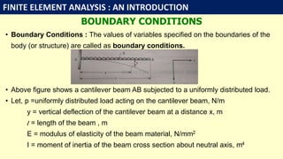
FUNDAMENTALS OF COMPUTER AIDED ENGINEERING
FINITE ELEMENT ANALYSIS : INTRODUCTION
UNIT III – FINITE ELEMENT ANALYSIS
By
Prof.(Dr) D Y Dhande
Professor
Department of Mechanical Engineering
AISSMS College Of Engineering, Pune – 411001
Email:dydhande@aissmscoe.com
FINITE ELEMENT ANALYSIS : AN INTRODUCTION
CONTENTS
• Need of finite element analysis
• Introduction to approaches used in Finite Element Analysis such as direct
approach and energy approach
• Boundary conditions: Types
• Rayleigh-Ritz Method
• Galerkin Method
FINITE ELEMENT ANALYSIS : AN INTRODUCTION
NEED OF FINITE ELEMENT ANALYSIS
• The Finite Element Analysis (FEA) is a numerical method for solving problems of
engineering and mathematical physics.
• Modern Mechanical design involves complicated shapes, sometimes made of different
materials.
• Useful for problems with complicated geometries, loadings, and material properties
where analytical solutions can not be obtained.
• The finite element analysis is based upon the idea of building a complicated object
into small pieces . Applications of the FEM can be found everywhere in day to day life
as well as engineering.
FINITE ELEMENT ANALYSIS : AN INTRODUCTION
FINITE ELEMENT METHOD
• In FEM, the body ( or structure) is divided into finite number of smaller units
known as elements. This process is known as discretization.
• Describe the behaviour of physical quantities on each element.
• Connect (assemble) the elements at the nodes to form an approximate
system of equations for the whole structure.
• Solve the system of equations involving unknown quantities at the nodes.
(e.g. displacements)
• Calculate desired quantities (strains and stresses) at selected elements.
FINITE ELEMENT ANALYSIS : AN INTRODUCTION
• Example :
FINITE ELEMENT ANALYSIS : AN INTRODUCTION
STAGES OF FINITE ELEMENT METHOD
Basic Steps:
• Discretization
• Selection of approximation of functions
• Formation of elemental stiffness matrix
• Formation of total stiffness matrix
• Formation of element loading matrix
• Formation of total loading matrix
• Formation of overall equilibrium equation
• Implementation of boundary condition
• Calculation of unknown nodal displacements
• Calculation of stresses and strains
FINITE ELEMENT ANALYSIS : AN INTRODUCTION
Phases:
• Pre–Processing:
Here a finite element mesh is developed to divide the given geometry into
subdomains for mathematical analysis and the material properties are
applied and also the boundary conditions.
• Solution:
In this phase governing matrix equations are derived and the solution for the
primary quantities is generated.
• Post-Processing:
In the last phase, checking of the validity of the solution generated ,
examination of the values of primary quantities such as displacement and
stresses, errors involved is carried out.
FINITE ELEMENT ANALYSIS : AN INTRODUCTION
ADVANTAGES OF FINITE ELEMENT ANALYSIS
• Can readily handle complex geometry.
• Can handle complex analysis types like vibration, heat transfer, fluids etc.
• Can handle complex loading:
i. Node-based loading (point loads).
ii. Element-based loading (pressure, thermal, inertial forces).
iii. Time or frequency dependent loading.
• Can handle complex restraints: Indeterminate structures can be analyzed.
• Can handle bodies comprised of nonhomogeneous materials: Can handle
bodies comprised of non-isotropic materials: Orthotropic & Anisotropic.
• Special material effects are handled such as temperature dependent
properties , plasticity , creep , swelling etc.
FINITE ELEMENT ANALYSIS : AN INTRODUCTION
LIMITATIONS OF FINITE ELEMENT ANALYSIS
• A specific numerical result is obtained for a specific problem.
• The FEM is applied to an approximation of the mathematical model of a system (the
source of so-called inherited errors).
• Experience and judgment are needed in order to construct a good finite element
model.
• A powerful computer and reliable FEM software are essential.
• Input and output data may be large and tedious to prepare and interpret.
• Numerical errors such as the limitation of the number of significant digits, rounding
–off occur very often.
• Fluid elements with boundaries at infinity can be computed and treated by using
boundary element method.
FINITE ELEMENT ANALYSIS : AN INTRODUCTION
APPLICATIONS OF FINITE ELEMENT ANALYSIS
• Mechanical/Aerospace/Civil/Automotive Engineering
• Structural/Stress Analysis
• Static/Dynamic
• Linear/Nonlinear
• Fluid Flow
• Heat Transfer
• Electromagnetic Fields
• Soil Mechanics
• Acoustics
• Biomechanics
FINITE ELEMENT ANALYSIS : AN INTRODUCTION
AVAILABLE COMMERCIAL SOFTWARE PACKAGES FOR FEM
• ANSYS
• NASTRAN
• PATRAN
• NISA / DISPLAY III
• LS DYNA
• HYPERMESH
• CATIA
• Pro-E(CREO)
• SOLID WORKS
• COSMOS
• COMSOL
• DYNA-3D
• ABAQUS
FINITE ELEMENT ANALYSIS : AN INTRODUCTION
BOUNDARY CONDITIONS
• Boundary Conditions : The values of variables specified on the boundaries of the
body (or structure) are called as boundary conditions.
• Above figure shows a cantilever beam AB subjected to a uniformly distributed load.
• Let, p =uniformly distributed load acting on the cantilever beam, N/m
y = vertical deflection of the cantilever beam at a distance x, m
= length of the beam , m
E = modulus of elasticity of the beam material, N/mm2
I = moment of inertia of the beam cross section about neutral axis, m4
l
FINITE ELEMENT ANALYSIS : AN INTRODUCTION
TYPES OF BOUNDARY CONDITIONS
• There are two types of boundary conditions :
(i) Geometric (Essential) boundary conditions
(ii) Force (Natural ) boundary conditions.
(1) Geometric (Essential) boundary conditions :
• In structural mechanics problems, the geometric or essential boundary conditions include
: specified displacements and slopes. The geometric or essential boundary conditions are
also known as kinematic boundary conditions.
• For above example, the geometric boundary conditions are:
At A (i.e. x = 0 ) are : displacement y = 0 and slope (dy/dx) = 0
(2) Force (Natural ) boundary conditions :
• In structural mechanics problems, the forced or natural boundary conditions include :
specified forces and moments. The force or natural boundary conditions are also known
as specified forces and moments. The force or natural boundary conditions are also
FINITE ELEMENT ANALYSIS : AN INTRODUCTION
known as static boundary conditions.
• Example of force boundary conditions: For above example, the force boundary conditions
at B ( i.e. X = l) are:
• Solution to Differential Equations:
• The solution to the differential equation must satisfy the above boundary conditions at A
and B as follows:
(i) the geometric boundary conditions at A (i.e. x = 0 )
(ii) the force boundary conditions at B ( i.e. X = l)
2
2
3
3
: 0
: 0
d y
bending moment EI
dx
d y
shear force EI
dx


FINITE ELEMENT ANALYSIS : AN INTRODUCTION
APPROXIMATE NUMERICAL METHODS
• For complex engineering problems, it is extremely difficult and many a times
impossible to obtain the exact analytical solution which satisfies all prescribed
boundary conditions.
• In such cases, approximate numerical methods are used as alternative methods of
finding solutions. These are:
( i) Variational ( Functional Approximation) Methods: Rayleigh- Ritz method and
Galerkin Method
(ii) Finite Element Method
(iii) Finite difference method.
FINITE ELEMENT ANALYSIS : AN INTRODUCTION

FEA: Analytical Methods.pptx

  • 2.
    FUNDAMENTALS OF COMPUTERAIDED ENGINEERING FINITE ELEMENT ANALYSIS : INTRODUCTION UNIT III – FINITE ELEMENT ANALYSIS
  • 3.
    By Prof.(Dr) D YDhande Professor Department of Mechanical Engineering AISSMS College Of Engineering, Pune – 411001 Email:dydhande@aissmscoe.com
  • 4.
    FINITE ELEMENT ANALYSIS: AN INTRODUCTION CONTENTS • Need of finite element analysis • Introduction to approaches used in Finite Element Analysis such as direct approach and energy approach • Boundary conditions: Types • Rayleigh-Ritz Method • Galerkin Method
  • 5.
    FINITE ELEMENT ANALYSIS: AN INTRODUCTION NEED OF FINITE ELEMENT ANALYSIS • The Finite Element Analysis (FEA) is a numerical method for solving problems of engineering and mathematical physics. • Modern Mechanical design involves complicated shapes, sometimes made of different materials. • Useful for problems with complicated geometries, loadings, and material properties where analytical solutions can not be obtained. • The finite element analysis is based upon the idea of building a complicated object into small pieces . Applications of the FEM can be found everywhere in day to day life as well as engineering.
  • 6.
    FINITE ELEMENT ANALYSIS: AN INTRODUCTION
  • 7.
    FINITE ELEMENT ANALYSIS: AN INTRODUCTION FINITE ELEMENT METHOD • In FEM, the body ( or structure) is divided into finite number of smaller units known as elements. This process is known as discretization. • Describe the behaviour of physical quantities on each element. • Connect (assemble) the elements at the nodes to form an approximate system of equations for the whole structure. • Solve the system of equations involving unknown quantities at the nodes. (e.g. displacements) • Calculate desired quantities (strains and stresses) at selected elements.
  • 8.
    FINITE ELEMENT ANALYSIS: AN INTRODUCTION • Example :
  • 9.
    FINITE ELEMENT ANALYSIS: AN INTRODUCTION STAGES OF FINITE ELEMENT METHOD Basic Steps: • Discretization • Selection of approximation of functions • Formation of elemental stiffness matrix • Formation of total stiffness matrix • Formation of element loading matrix • Formation of total loading matrix • Formation of overall equilibrium equation • Implementation of boundary condition • Calculation of unknown nodal displacements • Calculation of stresses and strains
  • 10.
    FINITE ELEMENT ANALYSIS: AN INTRODUCTION Phases: • Pre–Processing: Here a finite element mesh is developed to divide the given geometry into subdomains for mathematical analysis and the material properties are applied and also the boundary conditions. • Solution: In this phase governing matrix equations are derived and the solution for the primary quantities is generated. • Post-Processing: In the last phase, checking of the validity of the solution generated , examination of the values of primary quantities such as displacement and stresses, errors involved is carried out.
  • 11.
    FINITE ELEMENT ANALYSIS: AN INTRODUCTION
  • 12.
    FINITE ELEMENT ANALYSIS: AN INTRODUCTION ADVANTAGES OF FINITE ELEMENT ANALYSIS • Can readily handle complex geometry. • Can handle complex analysis types like vibration, heat transfer, fluids etc. • Can handle complex loading: i. Node-based loading (point loads). ii. Element-based loading (pressure, thermal, inertial forces). iii. Time or frequency dependent loading. • Can handle complex restraints: Indeterminate structures can be analyzed. • Can handle bodies comprised of nonhomogeneous materials: Can handle bodies comprised of non-isotropic materials: Orthotropic & Anisotropic. • Special material effects are handled such as temperature dependent properties , plasticity , creep , swelling etc.
  • 13.
    FINITE ELEMENT ANALYSIS: AN INTRODUCTION LIMITATIONS OF FINITE ELEMENT ANALYSIS • A specific numerical result is obtained for a specific problem. • The FEM is applied to an approximation of the mathematical model of a system (the source of so-called inherited errors). • Experience and judgment are needed in order to construct a good finite element model. • A powerful computer and reliable FEM software are essential. • Input and output data may be large and tedious to prepare and interpret. • Numerical errors such as the limitation of the number of significant digits, rounding –off occur very often. • Fluid elements with boundaries at infinity can be computed and treated by using boundary element method.
  • 14.
    FINITE ELEMENT ANALYSIS: AN INTRODUCTION APPLICATIONS OF FINITE ELEMENT ANALYSIS • Mechanical/Aerospace/Civil/Automotive Engineering • Structural/Stress Analysis • Static/Dynamic • Linear/Nonlinear • Fluid Flow • Heat Transfer • Electromagnetic Fields • Soil Mechanics • Acoustics • Biomechanics
  • 15.
    FINITE ELEMENT ANALYSIS: AN INTRODUCTION AVAILABLE COMMERCIAL SOFTWARE PACKAGES FOR FEM • ANSYS • NASTRAN • PATRAN • NISA / DISPLAY III • LS DYNA • HYPERMESH • CATIA • Pro-E(CREO) • SOLID WORKS • COSMOS • COMSOL • DYNA-3D • ABAQUS
  • 16.
    FINITE ELEMENT ANALYSIS: AN INTRODUCTION BOUNDARY CONDITIONS • Boundary Conditions : The values of variables specified on the boundaries of the body (or structure) are called as boundary conditions. • Above figure shows a cantilever beam AB subjected to a uniformly distributed load. • Let, p =uniformly distributed load acting on the cantilever beam, N/m y = vertical deflection of the cantilever beam at a distance x, m = length of the beam , m E = modulus of elasticity of the beam material, N/mm2 I = moment of inertia of the beam cross section about neutral axis, m4 l
  • 17.
    FINITE ELEMENT ANALYSIS: AN INTRODUCTION TYPES OF BOUNDARY CONDITIONS • There are two types of boundary conditions : (i) Geometric (Essential) boundary conditions (ii) Force (Natural ) boundary conditions. (1) Geometric (Essential) boundary conditions : • In structural mechanics problems, the geometric or essential boundary conditions include : specified displacements and slopes. The geometric or essential boundary conditions are also known as kinematic boundary conditions. • For above example, the geometric boundary conditions are: At A (i.e. x = 0 ) are : displacement y = 0 and slope (dy/dx) = 0 (2) Force (Natural ) boundary conditions : • In structural mechanics problems, the forced or natural boundary conditions include : specified forces and moments. The force or natural boundary conditions are also known as specified forces and moments. The force or natural boundary conditions are also
  • 18.
    FINITE ELEMENT ANALYSIS: AN INTRODUCTION known as static boundary conditions. • Example of force boundary conditions: For above example, the force boundary conditions at B ( i.e. X = l) are: • Solution to Differential Equations: • The solution to the differential equation must satisfy the above boundary conditions at A and B as follows: (i) the geometric boundary conditions at A (i.e. x = 0 ) (ii) the force boundary conditions at B ( i.e. X = l) 2 2 3 3 : 0 : 0 d y bending moment EI dx d y shear force EI dx  
  • 19.
    FINITE ELEMENT ANALYSIS: AN INTRODUCTION APPROXIMATE NUMERICAL METHODS • For complex engineering problems, it is extremely difficult and many a times impossible to obtain the exact analytical solution which satisfies all prescribed boundary conditions. • In such cases, approximate numerical methods are used as alternative methods of finding solutions. These are: ( i) Variational ( Functional Approximation) Methods: Rayleigh- Ritz method and Galerkin Method (ii) Finite Element Method (iii) Finite difference method.
  • 20.
    FINITE ELEMENT ANALYSIS: AN INTRODUCTION
  • 21.
    FINITE ELEMENT ANALYSIS: AN INTRODUCTION
  • 22.
    FINITE ELEMENT ANALYSIS: AN INTRODUCTION
  • 23.
    FINITE ELEMENT ANALYSIS: AN INTRODUCTION
  • 24.
    FINITE ELEMENT ANALYSIS: AN INTRODUCTION
  • 25.
    FINITE ELEMENT ANALYSIS: AN INTRODUCTION
  • 26.
    FINITE ELEMENT ANALYSIS: AN INTRODUCTION
  • 27.
    FINITE ELEMENT ANALYSIS: AN INTRODUCTION
  • 28.
    FINITE ELEMENT ANALYSIS: AN INTRODUCTION
  • 29.
    FINITE ELEMENT ANALYSIS: AN INTRODUCTION
  • 30.
    FINITE ELEMENT ANALYSIS: AN INTRODUCTION
  • 31.
    FINITE ELEMENT ANALYSIS: AN INTRODUCTION