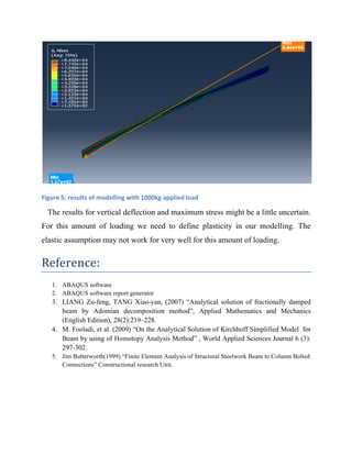
Finite Element Analysis (FEA) is a numerical method for solving complex engineering problems. The document discusses conducting FEA on a fixed-free cantilever beam to study the effect of mesh density on solution accuracy. Analytical solutions are derived and used to validate FEA results. A beam model is created in ABAQUS with varying element sizes. As element count increases, FEA results converge towards analytical solutions, though with increased computation time. An element count of 4125 provided an optimal balance between accuracy and cost.

1. Finite Element Analysis (FEA)
Ali tayebisadrabadi

2. INTRODUCTION
In order to consider the effects of new technologies in society we would like
to mention the advances in industry. Numerical modeling has a variety of
applications and offers an efficient method for solving highly complex
engineering problems. Techniques such as finite element analysis enable us to
assess complex problems for which analytical solutions are not feasible. We cannot
have the analytical solutions for complex problems; however, we can provide the
numerical solutions for them by modelling in finite element software [1, 2],
simulation with graphical software and many more options. The aim of this project
is to investigate the effects of mesh density in the accuracy of the finite element
solution.
The application of finite element methods requires an understanding of its
background, applications and methodologies. In this problem we want to study
loading of a fixed-free cantilever beam with respect to the effect of variations in
elements’ size [3]. Maybe it is not true but this parameter might be called the mesh
density. In order to conduct finite element analysis, an awareness of the
fundamentals of the software is required. In general, finite element analysis
includes the following steps [4]:
- Model creation
- Model idealisation
- Symmetries
- Meshing and discretisation (simplification of the problem)
- Specifying initial conditions and limitations
- Applying loading and boundary conditions
- Methods of solution

3. The above stages are common in finite element methods. However in the use of
specific finite element modelling software such as ABAQUS, further steps are
necessary as follows:
- Defining the type of analysis
- Creating or importing the geometry
- Defining material properties such as modulus of elasticity, poisson’s ratio
and any other required parameters
- Specifying mapped, sweep or simple meshing methods
- Follow the previous measured examples
- Post-processing of the model
- Extracting the desired results
Materials
&
Methods
In this report we will compare the results of analytical solutions with the results of
numerical modelling. The desired parameters for this model are the maximum
stress and the maximum deflection of the beam. Therefore, in the following
section, we will first describe the analytical solution of the model.
Analytical
Solution
Here, we have a fixed-free beam which is called a cantilever beam, and we would
like to study its behaviour upon applying vertical loading, assuming an elastic
model. We can imagine that on loading, due to deformation, we will have a
complete shape of a curve for beam. This would be because of this point that with
respect to the deformation in each point we will have a curved deflection for the

4. point of beam. We can derive the radius of this curvature from the two following
equations [5]:
!
!
=
!!!
!"!
[!!(
!"
!"
)!]!
!
1
𝑅
=
M(x)
EI
The first equation is derived from the equation of a curved function with
respect to 2D variation of its motion (planar assumption). And the second equation
is with respect to the elastic behaviour of the beam. It is a general formulation for
curved beams and we use it to define an analytical solution for this problem. With
respect to low variation in square of dy/dx relatively to 1, and the combination of
equations we will have for torque:
𝑀(𝑥) = EI
d
2
y
dx
2
If we consider this equation we will find that moment of each point relates to its
modulus of elasticity, second moment of inertia, and the second order derivative of
the shape function. These magnitudes vary for different locations. Now we can
easily find the maximum value for deflection at the end of the beam [5].
𝑣𝑒𝑟𝑡𝑖𝑐𝑎𝑙 𝑑𝑒𝑓𝑙𝑒𝑐𝑡𝑖𝑜𝑛 =
𝐹𝐿!
3𝐸𝐼
& 𝐹 = 𝑘𝑥 => 𝐾 = 3𝐸𝐼/𝐿!
Now if we consider the beam as a general linear spring with the equation of motion
F=kx, we can have the 3EI/L3
as the stiffness of the spring for the horizontal beam
in cantilever set up.

5. The second goal of this project is to use the results of the analytical solution for
maximum stress to investigate the accuracy of the numerical solution under
varying mesh densities. Therefore, we will setup our equations to find the
maximum available stress at the model.
For a general cantilever beam under different types of loading and
geometrical conditions, we will have the following conditions:
- Define the type of loading (axial, torsion, momentous, shear force, … )
- Detect the critical points
- Define the stresses due to different loadings
- Combine the stresses with a unique failure criteria method
- Define the most critical point (the maximum stress)
If we want to consider the general path of finding the maximum stress in loading
and conduct an indepth analysis of beams we need to follow a definite path.
However, in this project the focus is on maximum normal stress.
There are also another option for our analysis which is to consider the model as a
complete 2 dimensional model which is probably not incorrect for this problem.
However, there might be inevitable problem in magnitudes of stress from 2D to 3D
transformation.
When we apply a point load at the end of the beam it will have definite magnitudes
of stress at the fixed end due to moment and point vertical load transfers to the
area.
Therefore normal stress will be finally:
𝑛𝑜𝑟𝑚𝑎𝑙 𝑠𝑡𝑟𝑒𝑠𝑠 = ±
𝑀𝑐
𝐼
(+𝑓𝑜𝑟 𝑡𝑒𝑛𝑠𝑖𝑜𝑛 & − 𝑓𝑜𝑟 𝑐𝑜𝑚𝑝𝑟𝑒𝑠𝑠𝑖𝑜𝑛 )

6. There is also a transferred vertical point load at the fixed end which results
to shear stress which is:
𝑠ℎ𝑒𝑎𝑟 𝑠𝑡𝑟𝑒𝑠𝑠 = ±
𝑉𝑄
𝐼𝑡
𝑤ℎ𝑖𝑐ℎ 𝑚𝑖𝑔ℎ𝑡 𝑏𝑒 𝑛𝑒𝑔𝑙𝑖𝑔𝑎𝑏𝑙𝑒
However this shear stress is zero for free surface which have the highest
magnitude of normal stress. In the following, the results of the analytical solution
are presented, which will be useful in analysing of the numerical solution.
Analytical
calculation
In the previous section on analytical solution, the following equation was
derived. This is used for the calculation of vertical deflection and the x component
of stress.
𝑣𝑒𝑟𝑡𝑖𝑐𝑎𝑙 𝑑𝑒𝑓𝑙𝑒𝑐𝑡𝑖𝑜𝑛 𝑤𝑖𝑙𝑙 𝑏𝑒 𝑐𝑎𝑙𝑐𝑢𝑙𝑎𝑡𝑒𝑑 𝑡ℎ𝑟𝑜𝑢𝑔ℎ 𝑡ℎ𝑒 =
𝐹𝐿!
3𝐸𝐼
=
5 9.8 0.75 !
3 ∗ 113,800,000,000 ∗
1
12
∗ 0.001 ∗ 0.022!
= 0.068232
𝑎𝑛𝑑 𝑡ℎ𝑖𝑠 𝑤𝑖𝑙𝑙 𝑏𝑒 𝑐𝑜𝑛𝑡𝑖𝑛𝑢𝑒𝑑 𝑤𝑖𝑡ℎ 𝑥 𝑐𝑜𝑚𝑝𝑜𝑛𝑒𝑛𝑡 𝑜𝑓 𝑠𝑡𝑟𝑒𝑠𝑠 = = ±
𝐹𝐿𝑐
𝐼
= ±
5(9.8) 0.75 (0.022)/2
1
12
∗ 0.001 ∗ 0.022!
= 4.5558 𝑒8
Define
the
geometry
and
conditions
of
the
model:
There are many options for creating a geometrical model of the required
system. We can assume a complete 3D model or use a simpler 2D model and
specify its thickness. After creating the model, other options are specified in
modelling process, such as applying the elastic-plastic model conditions for the
beam and also defining a failure criterion for the model.

7. We would like to use a 2D or 3D model for simulating a fixed-free
cantilever beam. This will help us to produce a complete model for our
simulations. The behaviour of 2D & 3D models might have different results. This
will be possible for when we use a 2D model with real constant. Under this
condition, the element’s thickness will be imported into the analysis by the name
of real constant in 2D analysis. Therefore, the thickness term is not entered in
geometrical parameters. In this project we will describe the geometrical condition
of the model of our fixed-free cantilever beam in ABAQUS.
Figure
1:
the
given
2D
geometry
for
the
model
f
cantilever
beam
As it is obvious from the model we have a rectangular shape for the beam in
2D with 22*750 mm2
dimensions (Figure 1). The rectangular bar has the thickness
of 1 mm and therefore for the cross section of the beam we have another rectangle
of 1*22 mm2
. The left side is completely fixed and the right side is under a load of
5 kg, which will be considered as a point load in our modelling processes. Further
information on the beam is given in the following table:
Table1: material properties and beam characteristics
Fixed free cantilever Beam Magnitude of Parameters
Module of Elasticity 113.8 GPa
Poison Ratio 0.342 (dimensionless)
Ultimate tensile stress 950 MPa (14% strain rate considered)
Yield stress/ Engineering stress 880 MPa

8. The boundary conditions for this model are simple; with no displacement for
the fixed end and considering the middle axis of the beam to have no normal
tension (this is ideal assumption for 2D modelling).
Simulation,
Modelling
&
Results
In this research we will obtain the results for maximum vertical deflection,
maximum x component of stress, and also the time used for the process to be
solved with FEA. In this regard, we used ABAQUS commercial software to model
our geometry and will demonstrate the efficiency of the using ABAQUS software
for this project.
The following results will show the pictures of the model which are derived
under different mesh densities/ element numbers. By using smaller amounts for
element sizes the model can be idealized to higher number of elements. The
following table and the following figures can explain the conditions of the FEM
modeling and its results. As an example let us consider to the following table.
Table 1: information for the element types, numbers & etc...
Element Numbers Element Length Node numbers Element type
50 8.7234E+00 253 8-node linear brick, reduced
integration, hourglass control
280 5.2707E+00 1140 8-node linear brick, reduced
integration, hourglass control
1128 2.7187E+00 3969 8-node linear brick, reduced
integration, hourglass control
4125 1.5000E+00 13536 8-node linear brick, reduced
integration, hourglass control
11250 9.7407E-01 35682 8-node linear brick, reduced
integration, hourglass control

9. The following figure illustrates the variation in vertical deflection and x component
of stress in different locations along the modelled beam.
Figure
2:
results
of
a
model
with
280
elements
in
ABAQUS.
In the following figure we can observe the maximum and minimum magnitudes for
vertical deflection. This image is generated using the ABAQUS report generator
toolbox.
Figure
3:
The
figure
shows
that
maximum
and
minimum
magnitude
for
vertical
deflection
were
highlighted
for
the
model

10. There are also other parameters such as running time for the process, which might
be considered important. The following table demonstrates the time duration used
for each process.
# of elements Start time Finish time Used time
50 23:58:55 23:59:14 19
280 00:39:52 00:40:11 19
1128 00:59:26 00:59:46 20
4125 01:07:59 01:08:28 29
11250 01:16:01 01:16:59 58
The used time for different numbers of elements shows that we have a slight
increment for the used time of the process with increasing number of elements.
The derived data for the vertical deflection and x component of maximum stress is
given below. This is highly applicable for analysing the effects of mesh density
and changing element sizes.
Element numbers 50 280 1128 4125 11250
Vertical deflection (mm) 8.52e1 7.83e1 7.16e1 7.02e1 6.99e1
Von-mises stress 3.28e2 3.58e2 3.92e2 4.22e2 4.50e2
As it is obvious from the results of analytical solution that we need to increase our
element numbers. With increase in the number of elements, the results are in
better agreement with the analytical solution however, we will have more analysis
cost. Due to the greater time required for running the modelling process, we will
need to have a stronger processor. Therefore, it is very common to use a middle
point between these options, which might be called optimisation.

11.
Figure
4:
figure
shows
the
variation
of
different
parameters
with
changing
in
element
numbers
In this graph we can find the trend of different parameters with variation in number
of elements used in the FEM model. We can observe the variation in maximum
deflection in the vertical direction which increases and gets closer to its value in
the analytical solution. Therefore we find it that approximately 4125 could be the
optimum number of element to be used for this simple model in 1000 kg loading.
In the following section we will illustrate the results of applying 1000 kg loading
on the same simple beam after meshing with more than 4000 elements.
1000
kg
loading
on
simple
beam:
The results of applying 1000 kg load on the
same simple beam were generated as below:
- Characteristic element length 1.5000E+00
- Number of element 8250/2 = 4125 (we are using 8 node elements)
- Total number of nodes: 13536
- Maximum stress: 8.44e10 pa
- Vertical deflection: 1.4e4 mm
0
2
4
6
8
10
50
280
1128
4125
11250
process
/me/10
Maximum
stress
(X
component)*
e8
ver/cal
deflec/on
(mm)

12.
Figure
5:
results
of
modelling
with
1000kg
applied
load
The results for vertical deflection and maximum stress might be a little uncertain.
For this amount of loading we need to define plasticity in our modelling. The
elastic assumption may not work for very well for this amount of loading.
Reference:
1. ABAQUS software
2. ABAQUS software report generator
3. LIANG Zu-feng, TANG Xiao-yan, (2007) “Analytical solution of fractionally damped
beam by Adomian decomposition method”, Applied Mathematics and Mechanics
(English Edition), 28(2):219–228.
4. M. Fooladi, et al. (2009) “On the Analytical Solution of Kirchhoff Simplified Model for
Beam by using of Homotopy Analysis Method” , World Applied Sciences Journal 6 (3):
297-302.
5. Jim Butterworth(1999) “Finite Element Analysis of Structural Steelwork Beam to Column Bolted
Connections” Constructional research Unit.