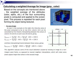
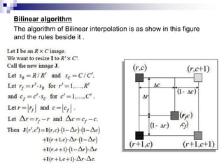
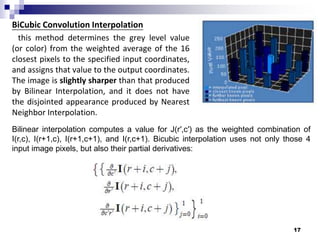
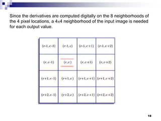
Digital image concepts and interpolation techniques for optical and digital zoom are discussed. There are three main types of interpolation used for resizing images: nearest neighbor, bilinear, and bicubic. Nearest neighbor is the simplest but produces the lowest quality, while bicubic is the most complex but highest quality. Optical zoom uses lens magnification before sensing, whereas digital zoom interpolates after sensing, resulting in lower quality than optical zoom. Interpolation methods assign pixel values to new locations during resizing based on weighting patterns around the original pixel values.

1. 1
Image Interpolation Techniques
with
Optical and Digital Zoom
Concepts
Musaab M. Jasim
Yildiz Technical University
Computer department
Seminar

2. 2
Outline
 Digital Image concepts .
 Digital Image definition .
 Image Acquisition Using Sensor Arrays .
 Basic Concepts in Sampling and Quantization .
 Digital Image Clarity.
 Optical Zoom vs. Digital Zoom .
 Image Interpolation (spatial processing).
 Nearest Neighbor .
 Bilinear .
 Bicubic.
 Conclusion.

3. Digital Image concepts
Digital Image Definition
 The digital Image is a visual representation in form of a function f(x,y)
where “ f ” is Intensity value (bit depth) and it is related to the brightness
(or color) at point (x,y) .
 The value of each point is acquired based on the light that reflect from
the objects on the sensors inside the Digital Camera .
3
Right idea Wrong idea

4. Image Acquisition Using Sensors Array
 Sensors arranged in the form of a 2-D array.
 The light that reflect from the objects on the sensors will be aggregated.
4

5. Basic Concepts in Sampling and Quantization
 The result of sensor array (acquisition process) is an image which be
continuous with respect to the x , y-coordinates, and also in amplitude.
 Digitizing the coordinate values is called sampling .
 Digitizing the amplitude values is called quantization.
5

6. Basic Concepts in Sampling and Quantization
 after the sampling and quantization processes the image pixels will
been created
6
Continues Image on
sensor array
Digital image

7. 7
Digital Image Clarity
 A Pixel is actually a unit of the digital image .
 A Resolution is the capability of the sensor to observe or measure the
smallest object clearly with distinct boundaries.
 the Resolution is the measurement unit of the clarity in digital image .
 There are three types of resolution:
I. the Pixel Resolution determine the number of pixels in the image .(related
with the size of the pixel).
but unfortunately, the count of pixels isn't a real measure of the image clarity
as most people think . There are another resolution types affects.
II. The Spatial Resolution can be defined as the number of independent pixel
values per unit length .
III. The Intensity Resolution is the bit depth or the colors range of pixels in image.

8. 8
Optical Zoom vs. Digital Zoom
 An Optical zoom means moving the zoom lens so that it increases the
magnification of light before it even reaches the digital sensor.
 A digital zoom is not really zoom , it is simply interpolating the image
after it has been acquired at the sensor (pixilation process).
Original image
Optical
Zooming
Digital
Zooming

9. 9
Image Interpolation (spatial processing).
 Image resizing is necessary when we need to increase or decrease the
total number of pixels .
 so it mean resampling the image by creating new pixel locations and
assigning gray-level values (or color) to these locations.
 There are two types of resizing methods
A. Adaptive .(beyond my presentation)
B. Non-adaptive :
A. Nearest Neighbor interpolation.
B. Bilinear interpolation .
C. Bicubic interpolation .
 Image interpolation occurs
when we resize or distort our
image from one pixel grid to
another.

10. 10
Nearest Neighbor Interpolation
 the simplest method, determines the grey level value(or color) from the
closest pixel to the specified input coordinates, and assigns that value
to the output coordinates.
Enlargement Reduction

11. 11
Nearest Neighbor Algorithm
 This algorithm assumed that :
 (R=r+1 and C=c+1). So, 𝑆 𝑟, 𝑆𝑐 has two
states .
 Some conditions to delete the frame.
 In another Image processing books
, It assumed that the:
 (R=r and C=c). So, 𝑆 𝑟, 𝑆𝑐 has just the first
state .
 This what I assumed in my Example to
facilitate it.

12. 12
Nearest Neighbor Example
(1,1) (1,2) (1,3) (1,4)
(2,1) (2,2) (2,3) (2,4)
(3,1) (3,2) (3,3) (3,4)
(4,1) (4,2) (4,3) (4,4)
I (R X C) =
(1,1) (1,2) (1,3) (1,4) (1,5) (1,6) (1,7) (1,8)
(2,1) (2,2) (2,3) (2,4) (2,5) (2,6) (2,7) (2,8)
(3,1) (3,2) (3,3) (3,4) (3,5) (3,6) (3,7) (3,8)
(4,1) (4,2) (4,3) (4,4) (4,5) (4,6) (4,7) (4,8)
(5,1) (5,2) (5,3) (5,4) (5,5) (5,6) (5,7) (5,8)
(6,1) (6,2) (6,3) (6,4) (6,5) (6,6) (6,7) (6,8)
(7,1) (7,2) (7,3) (7,4) (7,5) (7,6) (7,7) (7,8)
(8,1) (8,2) (8,3) (8,4) (8,5) (8,6) (8,7) (8,8)
J ( 𝑅 𝐗 𝐶) =
𝑆 𝑟=
𝑅
𝑅
𝑆 𝐶=
𝐶
𝐶
= 0.5 = 0.5
(𝑟𝑓 , 𝑐 𝑓) = (𝑆 𝑟∗ 𝑟 , 𝑆𝑐∗ 𝑐 ) =
R=r & C=c
(0.5 , 0.5) (0.5 , 1) (0.5 , 1.5) (0.5 , 2) (0.5 , 2.5) (0.5 , 3) (0.5 , 3.5) (0.5 , 4)
(1 , 0.5) (1 , 1) (1,1.5) (1,2) (1,2.5) (1,3) (1,3.5) (1,4)
(1.5,0.5) (1.5 , 1) (1.5,1.5) (1.5,2) (1.5,2.5) (1.5,3) (1.5,3.5) (1.5,4)
(2 , 0.5) (2 , 1) (2,1.5) (2,2) (2,2.5) (2,3) (2,3.5) (2,4)
(2.5 , 0.5) (2.5 , 1) (2.5,1.5) (2.5,2) (2.5,2.5) (2.5,3) (2.5,3.5) (2.5,4)
(3,0.5) (3 , 1) (3,1.5) (3,2) (3,2.5) (3,3) (3,3.5) (3,4)
(3.5 , 0.5) (3.5 , 1) (3.5,1.5) (3.5,2) (3.5,2.5) (3.5,3) (3.5,3.5) (3.5,4)
(4 , 0.5) (4 , 1) (4,1.5) (4,2) (4,2.5) (4,3) (4,3.5) (4,4)
(𝑟 , 𝑐) = 𝑅𝑜𝑢𝑛𝑑{ 𝑟𝑓 , 𝑐 𝑓 } =
(1 , 1) (1 , 1) (1,2) (1 , 2) (1 , 3) (1 , 3) (1 , 4) (1 , 4)
(1 , 1) (1 , 1) (1,2) (1,2) (1,3) (1,3) (14) (1,4)
(2,1) (2 , 1) (2,2) (2,2) (2,3) (2,3) (2,4) (2,4)
(2 , 1) (2 , 1) (2,2) (2,2) (2,3) (2,3) (2,4) (2,4)
(3 , 1) (3 , 1) (3,2) (3,2) (3,3) (3,3) (3,4) (3,4)
(3,1) (3 , 1) (3,2) (3,2) (3,3) (3,3) (3,4) (3,4)
(4 , 1) (4 , 1) (4,2) (4,2) (4,3) (4,3) (4,3.5) (4,4)
(4 , 1) (4 , 1) (4,2) (4,2) (4,3) (4,3) (4,4) (4,4)
𝐽( 𝑟, 𝑐) = I (𝑟 , 𝑐)

13. 13
Bilinear Interpolation
 Bilinear Interpolation determines the grey level value (or color) from the
weighted average of the four closest pixels to the specified input
coordinates, and assigns that value to the output coordinates.
Linear interpolation between two known points
Interpolation is the process of estimating the values of a continuous function from
discrete samples.
𝑦 − 𝑦0
𝑥 − 𝑥0
=
𝑦1 − 𝑦0
𝑥1 − 𝑥0
𝑦 = 𝑦0 + 𝑦1 − 𝑦0 ∗
𝑥 − 𝑥0
𝑥1 − 𝑥0

14. 14
Bilinear Interpolation
weighted average
• The previews formula can also be understood as a weighted average .
• The closer point has more influence than the farther point. Thus, the weights are
𝑥−𝑥0
𝑥1−𝑥0
and 𝑥1−𝑥
𝑥1−𝑥0
which are normalized distances between the unknown point and
each of the end points.
𝑦 = 𝑦0 1 − 𝑥−𝑥0
𝑥1−𝑥0
+ 𝑦1 1 − 𝑥1−𝑥
𝑥1−𝑥0
= 𝑦 = 𝑦0 1 − 𝑥−𝑥0
𝑥1−𝑥0
+ 𝑦1
𝑥−𝑥0
𝑥1−𝑥0

15. 15
Bilinear Interpolation
Example
• we observe that the intensity value at the pixel computed to be at row 20.2,
column 14.5 can be calculated by first linearly interpolating between the values
at column 14 and 15 on each rows 20 and 21, giving
𝐼20,14.5 =
15 − 14.5
15 − 14
∗ 91 +
14.5 − 14
15 − 14
∗ 210 = 150.5
𝐼21,14.5 =
15 − 14.5
15 − 14
∗ 162 +
14.5 − 14
15 − 14
∗ 95 = 128.5
and then interpolating linearly between these values, giving
𝐼20.2 ,14.5 =
21 − 20.2
21 − 20
∗ 150.5 +
20.2 − 20
21 − 20
∗ 128.5 = 146.1

16. 16
Bilinear Algorithm

17. 17
Bicubic Interpolation
 BiCubic Interpolation method determines the gray level value (or color)
from the weighted average of the 16 closest pixels to the specified input
coordinates .
 The image is sharper and more clarity than that produced by Nearest
neighbor and Bilinear Interpolation .
 It needs much more calculation and time to find weighting..

18. Conclusion
 The digital images are result of the optical intensity that is received at
the image plane (Sensor array) inside a digital camera .
 Digital Zooming includes : enlargement and shrinking processes where
these processes require two steps: the creation of new pixel locations,
and the assignment of gray (or color) levels to those new locations .
 Descending order for the methods of zooming with respect to the
picture quality, processing time is :
i. Bicubic Interpolation .
ii. Bilinear Interpolation .
iii. Nearest Neighbor Interpolation .
18

19. The end
“ thank you to all attendees “
19