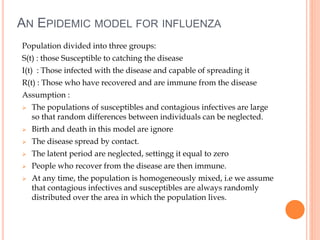
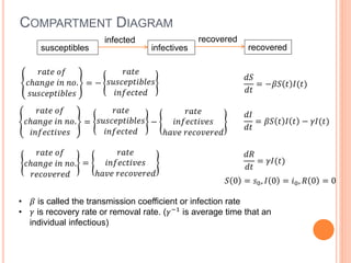
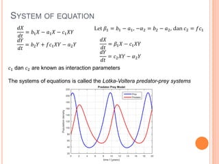
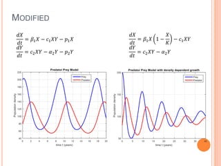
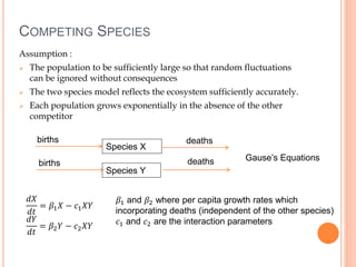
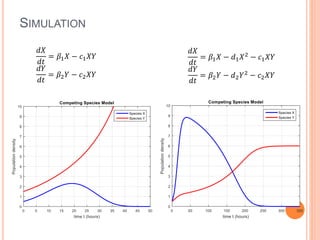
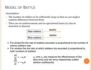
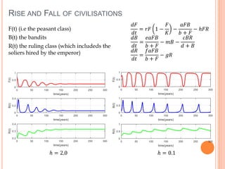
INTERACTING POPULATION MODELS
Pengajar :
Heni Widayani, M.Si
Senin, 20 Februari 2018
MATA KULIAH:
PEMODELAN MATEMATIKA
AN EPIDEMIC MODEL FOR INFLUENZA
Population divided into three groups:
S(t) : those Susceptible to catching the disease
I(t) : Those infected with the disease and capable of spreading it
R(t) : Those who have recovered and are immune from the disease
Assumption :
 The populations of susceptibles and contagious infectives are large
so that random differences between individuals can be neglected.
 Birth and death in this model are ignore
 The disease spread by contact.
 The latent period are neglected, settingg it equal to zero
 People who recover from the disease are then immune.
 At any time, the population is homogeneously mixed, i.e we assume
that contagious infectives and susceptibles are always randomly
distributed over the area in which the population lives.
COMPARTMENT DIAGRAM
infectives recoveredsusceptibles
recoveredinfected
𝑟𝑎𝑡𝑒 𝑜𝑓
𝑐ℎ𝑎𝑛𝑔𝑒 𝑖𝑛 𝑛𝑜.
𝑠𝑢𝑠𝑐𝑒𝑝𝑡𝑖𝑏𝑙𝑒𝑠
= −
𝑟𝑎𝑡𝑒
𝑠𝑢𝑠𝑐𝑒𝑝𝑡𝑖𝑏𝑙𝑒𝑠
𝑖𝑛𝑓𝑒𝑐𝑡𝑒𝑑
𝑟𝑎𝑡𝑒 𝑜𝑓
𝑐ℎ𝑎𝑛𝑔𝑒 𝑖𝑛 𝑛𝑜.
𝑖𝑛𝑓𝑒𝑐𝑡𝑖𝑣𝑒𝑠
=
𝑟𝑎𝑡𝑒
𝑠𝑢𝑠𝑐𝑒𝑝𝑡𝑖𝑏𝑙𝑒𝑠
𝑖𝑛𝑓𝑒𝑐𝑡𝑒𝑑
−
𝑟𝑎𝑡𝑒
𝑖𝑛𝑓𝑒𝑐𝑡𝑖𝑣𝑒𝑠
ℎ𝑎𝑣𝑒 𝑟𝑒𝑐𝑜𝑣𝑒𝑟𝑒𝑑
𝑟𝑎𝑡𝑒 𝑜𝑓
𝑐ℎ𝑎𝑛𝑔𝑒 𝑖𝑛 𝑛𝑜.
𝑟𝑒𝑐𝑜𝑣𝑒𝑟𝑒𝑑
=
𝑟𝑎𝑡𝑒
𝑖𝑛𝑓𝑒𝑐𝑡𝑖𝑣𝑒𝑠
ℎ𝑎𝑣𝑒 𝑟𝑒𝑐𝑜𝑣𝑒𝑟𝑒𝑑
𝑑𝑆
𝑑𝑡
= −𝛽𝑆 𝑡 𝐼(𝑡)
𝑑𝐼
𝑑𝑡
= 𝛽𝑆 𝑡 𝐼 𝑡 − 𝛾𝐼(𝑡)
𝑑𝑅
𝑑𝑡
= 𝛾𝐼(𝑡)
• 𝛽 is called the transmission coefficient or infection rate
• 𝛾 is recovery rate or removal rate. (𝛾−1
is average time that an
individual infectious)
𝑆 0 = 𝑠0, 𝐼 0 = 𝑖0, 𝑅 0 = 0
THE BASIC REPRODUCTION NUMBER
The basic reproduction number 𝑅0 is defined as the number of new
secondary infections resulting from a single infectious individual placed in a
completely susceptible population, over the time that individual is infectious.
If 𝑅0 < 1 we would expect the disease outbreak to die out (I(t) to decrease)
If 𝑅0 > 1 then it would increase initially
SIMULATION
𝑅0 =
𝛽𝑆(0)
𝛾
If we vaccinate a proportion 𝑝 of the population of susceptible then this
means that the basic reproduction number changes to
𝑅 𝑣 =
1 − 𝑝 𝛽𝑆(0)
𝛾
= (1 − 𝑝)𝑅0
To eradicate the disease, 𝑅 𝑣 < 1, then 𝑝 > 1 −
1
𝑅0
.
ENDEMIC DISEASE
𝑎 denote the natural per capita death rate of population
𝑏 denote the natural per capita birth rate of population
𝑁 𝑡 = 𝑆 𝑡 + 𝐼 𝑡 + 𝑅 𝑡
𝑑𝑁
𝑑𝑡
= 𝑏 − 𝑎 𝑁
If 𝑏 = 𝑎 the the population remains constant.
I(t) R(t)S(t)
recoveredinfectedbirths
deaths deaths deaths
𝑑𝑆
𝑑𝑡
= 𝑏𝑁 − 𝛽𝑆𝐼 − 𝑎𝑆
𝑑𝐼
𝑑𝑡
= 𝛽𝑆𝐼 − 𝛾𝐼 − 𝑎𝐼
𝑑𝑅
𝑑𝑡
= 𝛾𝐼 − 𝑎𝑅
PREDATORS AND PREY
Assumption :
 The population are large, sufficiently large to neglect random
differences between individuals.
 The effect of pestiside initially are ignored
 There are only two populations, the predator and the prey, which
affect the ecosystem.
 The prey population grows exponentially in the absence of predator.
PREY
PREDATORS
Natural births
births
Natural deaths
Deaths from predators
Natural deaths
SYSTEM OF EQUATION
Let 𝛽1 = 𝑏1 − 𝑎1, −𝛼2 = 𝑏2 − 𝑎2, dan 𝑐2 = 𝑓𝑐1𝑑𝑋
𝑑𝑡
= 𝑏1 𝑋 − 𝑎1 𝑋 − 𝑐1 𝑋𝑌
𝑑𝑌
𝑑𝑡
= 𝑏2 𝑌 + 𝑓𝑐1 𝑋𝑌 − 𝑎2 𝑌
𝑑𝑋
𝑑𝑡
= 𝛽1 𝑋 − 𝑐1 𝑋𝑌
𝑑𝑌
𝑑𝑡
= 𝑐2 𝑋𝑌 − 𝛼2 𝑌
𝑐1 dan 𝑐2 are known as interaction parameters
The systems of equations is called the Lotka-Voltera predator-prey systems
MODIFIED
𝑑𝑋
𝑑𝑡
= 𝛽1 𝑋 − 𝑐1 𝑋𝑌 − 𝑝1 𝑋
𝑑𝑌
𝑑𝑡
= 𝑐2 𝑋𝑌 − 𝛼2 𝑌 − 𝑝2 𝑌
𝑑𝑋
𝑑𝑡
= 𝛽1 𝑋 1 −
𝑋
𝐾
− 𝑐1 𝑋𝑌
𝑑𝑌
𝑑𝑡
= 𝑐2 𝑋𝑌 − 𝛼2 𝑌
COMPETING SPECIES
Assumption :
 The population to be sufficiently large so that random fluctuations
can be ignored without consequences
 The two species model reflects the ecosystem sufficiently accurately.
 Each population grows exponentially in the absence of the other
competitor
Species X
Species Y
births
births deaths
deaths
𝑑𝑋
𝑑𝑡
= 𝛽1 𝑋 − 𝑐1 𝑋𝑌
𝑑𝑌
𝑑𝑡
= 𝛽2 𝑌 − 𝑐2 𝑋𝑌
𝛽1 and 𝛽2 where per capita growth rates which
incorporating deaths (independent of the other species)
𝑐1 and 𝑐2 are the interaction parameters
Gause’s Equations
SIMULATION
𝑑𝑋
𝑑𝑡
= 𝛽1 𝑋 − 𝑐1 𝑋𝑌
𝑑𝑌
𝑑𝑡
= 𝛽2 𝑌 − 𝑐2 𝑋𝑌
𝑑𝑋
𝑑𝑡
= 𝛽1 𝑋 − 𝑑1 𝑋2 − 𝑐1 𝑋𝑌
𝑑𝑌
𝑑𝑡
= 𝛽2 𝑌 − 𝑑2 𝑌2 − 𝑐2 𝑋𝑌
MODEL OF BATTLE
Assumption :
 The number of soldiers to be sufficiently large so that we can neglect
random differences between them
 There are no reinforcements and no operational losses (i.e due to
desertion or disease)
Red soldiers
Blue soldiers
deaths
deaths
 For aimed fire the rate of soldiers wounded is proportional to the number of
enemy soldiers only
 For random fire the rate at which soldiers are wounded is proportional to
both numbers of soldiers
𝑑𝑅
𝑑𝑡
= −𝑎1 𝐵
𝑑𝐵
𝑑𝑡
= −𝑎2 𝑅
𝑎1 and 𝑎2 are measure the effectiveness of the
blue army and red army respectively (called
attrition coefficients)
SIMULATION
𝑑𝑅
𝑑𝑡
= −𝑎1 𝐵
𝑑𝐵
𝑑𝑡
= −𝑎2 𝑅
𝑑𝑅
𝑑𝑡
= −𝑎1 𝐵
𝑑𝐵
𝑑𝑡
= −𝑐2 𝑅𝐵
𝑑𝑅
𝑑𝑡
= −𝑐1 𝑅𝐵
𝑑𝐵
𝑑𝑡
= −𝑐2 𝑅𝐵
RISE AND FALL OF CIVILISATIONS
F(t) (i.e the peasant class)
B(t) the bandits
R(t) the ruling class (which includeds the
soliers hired by the emperor)
𝑑𝐹
𝑑𝑡
= 𝑟𝐹 1 −
𝐹
𝐾
−
𝑎𝐹𝐵
𝑏 + 𝐹
− ℎ𝐹𝑅
𝑑𝐵
𝑑𝑡
=
𝑒𝑎𝐹𝐵
𝑏 + 𝐹
− 𝑚𝐵 −
𝑐𝐵𝑅
𝑑 + 𝐵
𝑑𝑅
𝑑𝑡
=
𝑓𝑎𝐹𝐵
𝑏 + 𝐹
− 𝑔𝑅
ℎ = 2.0 ℎ = 0.1

Interacting Population Models

  • 1.
    INTERACTING POPULATION MODELS Pengajar: Heni Widayani, M.Si Senin, 20 Februari 2018 MATA KULIAH: PEMODELAN MATEMATIKA
  • 2.
    AN EPIDEMIC MODELFOR INFLUENZA Population divided into three groups: S(t) : those Susceptible to catching the disease I(t) : Those infected with the disease and capable of spreading it R(t) : Those who have recovered and are immune from the disease Assumption :  The populations of susceptibles and contagious infectives are large so that random differences between individuals can be neglected.  Birth and death in this model are ignore  The disease spread by contact.  The latent period are neglected, settingg it equal to zero  People who recover from the disease are then immune.  At any time, the population is homogeneously mixed, i.e we assume that contagious infectives and susceptibles are always randomly distributed over the area in which the population lives.
  • 3.
    COMPARTMENT DIAGRAM infectives recoveredsusceptibles recoveredinfected 𝑟𝑎𝑡𝑒𝑜𝑓 𝑐ℎ𝑎𝑛𝑔𝑒 𝑖𝑛 𝑛𝑜. 𝑠𝑢𝑠𝑐𝑒𝑝𝑡𝑖𝑏𝑙𝑒𝑠 = − 𝑟𝑎𝑡𝑒 𝑠𝑢𝑠𝑐𝑒𝑝𝑡𝑖𝑏𝑙𝑒𝑠 𝑖𝑛𝑓𝑒𝑐𝑡𝑒𝑑 𝑟𝑎𝑡𝑒 𝑜𝑓 𝑐ℎ𝑎𝑛𝑔𝑒 𝑖𝑛 𝑛𝑜. 𝑖𝑛𝑓𝑒𝑐𝑡𝑖𝑣𝑒𝑠 = 𝑟𝑎𝑡𝑒 𝑠𝑢𝑠𝑐𝑒𝑝𝑡𝑖𝑏𝑙𝑒𝑠 𝑖𝑛𝑓𝑒𝑐𝑡𝑒𝑑 − 𝑟𝑎𝑡𝑒 𝑖𝑛𝑓𝑒𝑐𝑡𝑖𝑣𝑒𝑠 ℎ𝑎𝑣𝑒 𝑟𝑒𝑐𝑜𝑣𝑒𝑟𝑒𝑑 𝑟𝑎𝑡𝑒 𝑜𝑓 𝑐ℎ𝑎𝑛𝑔𝑒 𝑖𝑛 𝑛𝑜. 𝑟𝑒𝑐𝑜𝑣𝑒𝑟𝑒𝑑 = 𝑟𝑎𝑡𝑒 𝑖𝑛𝑓𝑒𝑐𝑡𝑖𝑣𝑒𝑠 ℎ𝑎𝑣𝑒 𝑟𝑒𝑐𝑜𝑣𝑒𝑟𝑒𝑑 𝑑𝑆 𝑑𝑡 = −𝛽𝑆 𝑡 𝐼(𝑡) 𝑑𝐼 𝑑𝑡 = 𝛽𝑆 𝑡 𝐼 𝑡 − 𝛾𝐼(𝑡) 𝑑𝑅 𝑑𝑡 = 𝛾𝐼(𝑡) • 𝛽 is called the transmission coefficient or infection rate • 𝛾 is recovery rate or removal rate. (𝛾−1 is average time that an individual infectious) 𝑆 0 = 𝑠0, 𝐼 0 = 𝑖0, 𝑅 0 = 0
  • 4.
    THE BASIC REPRODUCTIONNUMBER The basic reproduction number 𝑅0 is defined as the number of new secondary infections resulting from a single infectious individual placed in a completely susceptible population, over the time that individual is infectious. If 𝑅0 < 1 we would expect the disease outbreak to die out (I(t) to decrease) If 𝑅0 > 1 then it would increase initially
  • 5.
    SIMULATION 𝑅0 = 𝛽𝑆(0) 𝛾 If wevaccinate a proportion 𝑝 of the population of susceptible then this means that the basic reproduction number changes to 𝑅 𝑣 = 1 − 𝑝 𝛽𝑆(0) 𝛾 = (1 − 𝑝)𝑅0 To eradicate the disease, 𝑅 𝑣 < 1, then 𝑝 > 1 − 1 𝑅0 .
  • 6.
    ENDEMIC DISEASE 𝑎 denotethe natural per capita death rate of population 𝑏 denote the natural per capita birth rate of population 𝑁 𝑡 = 𝑆 𝑡 + 𝐼 𝑡 + 𝑅 𝑡 𝑑𝑁 𝑑𝑡 = 𝑏 − 𝑎 𝑁 If 𝑏 = 𝑎 the the population remains constant. I(t) R(t)S(t) recoveredinfectedbirths deaths deaths deaths 𝑑𝑆 𝑑𝑡 = 𝑏𝑁 − 𝛽𝑆𝐼 − 𝑎𝑆 𝑑𝐼 𝑑𝑡 = 𝛽𝑆𝐼 − 𝛾𝐼 − 𝑎𝐼 𝑑𝑅 𝑑𝑡 = 𝛾𝐼 − 𝑎𝑅
  • 7.
    PREDATORS AND PREY Assumption:  The population are large, sufficiently large to neglect random differences between individuals.  The effect of pestiside initially are ignored  There are only two populations, the predator and the prey, which affect the ecosystem.  The prey population grows exponentially in the absence of predator. PREY PREDATORS Natural births births Natural deaths Deaths from predators Natural deaths
  • 8.
    SYSTEM OF EQUATION Let𝛽1 = 𝑏1 − 𝑎1, −𝛼2 = 𝑏2 − 𝑎2, dan 𝑐2 = 𝑓𝑐1𝑑𝑋 𝑑𝑡 = 𝑏1 𝑋 − 𝑎1 𝑋 − 𝑐1 𝑋𝑌 𝑑𝑌 𝑑𝑡 = 𝑏2 𝑌 + 𝑓𝑐1 𝑋𝑌 − 𝑎2 𝑌 𝑑𝑋 𝑑𝑡 = 𝛽1 𝑋 − 𝑐1 𝑋𝑌 𝑑𝑌 𝑑𝑡 = 𝑐2 𝑋𝑌 − 𝛼2 𝑌 𝑐1 dan 𝑐2 are known as interaction parameters The systems of equations is called the Lotka-Voltera predator-prey systems
  • 9.
    MODIFIED 𝑑𝑋 𝑑𝑡 = 𝛽1 𝑋− 𝑐1 𝑋𝑌 − 𝑝1 𝑋 𝑑𝑌 𝑑𝑡 = 𝑐2 𝑋𝑌 − 𝛼2 𝑌 − 𝑝2 𝑌 𝑑𝑋 𝑑𝑡 = 𝛽1 𝑋 1 − 𝑋 𝐾 − 𝑐1 𝑋𝑌 𝑑𝑌 𝑑𝑡 = 𝑐2 𝑋𝑌 − 𝛼2 𝑌
  • 10.
    COMPETING SPECIES Assumption : The population to be sufficiently large so that random fluctuations can be ignored without consequences  The two species model reflects the ecosystem sufficiently accurately.  Each population grows exponentially in the absence of the other competitor Species X Species Y births births deaths deaths 𝑑𝑋 𝑑𝑡 = 𝛽1 𝑋 − 𝑐1 𝑋𝑌 𝑑𝑌 𝑑𝑡 = 𝛽2 𝑌 − 𝑐2 𝑋𝑌 𝛽1 and 𝛽2 where per capita growth rates which incorporating deaths (independent of the other species) 𝑐1 and 𝑐2 are the interaction parameters Gause’s Equations
  • 11.
    SIMULATION 𝑑𝑋 𝑑𝑡 = 𝛽1 𝑋− 𝑐1 𝑋𝑌 𝑑𝑌 𝑑𝑡 = 𝛽2 𝑌 − 𝑐2 𝑋𝑌 𝑑𝑋 𝑑𝑡 = 𝛽1 𝑋 − 𝑑1 𝑋2 − 𝑐1 𝑋𝑌 𝑑𝑌 𝑑𝑡 = 𝛽2 𝑌 − 𝑑2 𝑌2 − 𝑐2 𝑋𝑌
  • 12.
    MODEL OF BATTLE Assumption:  The number of soldiers to be sufficiently large so that we can neglect random differences between them  There are no reinforcements and no operational losses (i.e due to desertion or disease) Red soldiers Blue soldiers deaths deaths  For aimed fire the rate of soldiers wounded is proportional to the number of enemy soldiers only  For random fire the rate at which soldiers are wounded is proportional to both numbers of soldiers 𝑑𝑅 𝑑𝑡 = −𝑎1 𝐵 𝑑𝐵 𝑑𝑡 = −𝑎2 𝑅 𝑎1 and 𝑎2 are measure the effectiveness of the blue army and red army respectively (called attrition coefficients)
  • 13.
    SIMULATION 𝑑𝑅 𝑑𝑡 = −𝑎1 𝐵 𝑑𝐵 𝑑𝑡 =−𝑎2 𝑅 𝑑𝑅 𝑑𝑡 = −𝑎1 𝐵 𝑑𝐵 𝑑𝑡 = −𝑐2 𝑅𝐵 𝑑𝑅 𝑑𝑡 = −𝑐1 𝑅𝐵 𝑑𝐵 𝑑𝑡 = −𝑐2 𝑅𝐵
  • 14.
    RISE AND FALLOF CIVILISATIONS F(t) (i.e the peasant class) B(t) the bandits R(t) the ruling class (which includeds the soliers hired by the emperor) 𝑑𝐹 𝑑𝑡 = 𝑟𝐹 1 − 𝐹 𝐾 − 𝑎𝐹𝐵 𝑏 + 𝐹 − ℎ𝐹𝑅 𝑑𝐵 𝑑𝑡 = 𝑒𝑎𝐹𝐵 𝑏 + 𝐹 − 𝑚𝐵 − 𝑐𝐵𝑅 𝑑 + 𝐵 𝑑𝑅 𝑑𝑡 = 𝑓𝑎𝐹𝐵 𝑏 + 𝐹 − 𝑔𝑅 ℎ = 2.0 ℎ = 0.1