This document discusses image enhancement techniques in the spatial domain. It describes two categories of spatial domain operations: point processing and neighborhood processing. Point processing involves direct manipulation of pixel values through techniques like contrast stretching and thresholding. Neighborhood processing considers pixels in a local region and applies techniques like averaging filters. The document outlines several gray level transformations for enhancement, including logarithmic, power-law, piecewise linear, and bit-plane slicing transformations. It also discusses arithmetic and logic operations on images.

1. Chap. 3: Image Enhancement
in the Spatial Domain

2. Image Enhancement
 Goal: process an image so that the result is
more suitable than the original image for a
specific application
 Visual interpretation
 Problem oriented

3. Image enhancement example

4. Two categories
 There is no general theory of image
enhancement
 Spatial domain
 Direct manipulation of pixels
 Point processing
 Neighborhood processing
 Frequency domain
 Modify the Fourier transform of an image

5. Outline: spatial domain
operations
 Background
 Gray level transformations
 Arithmetic/logic operations

6. Background
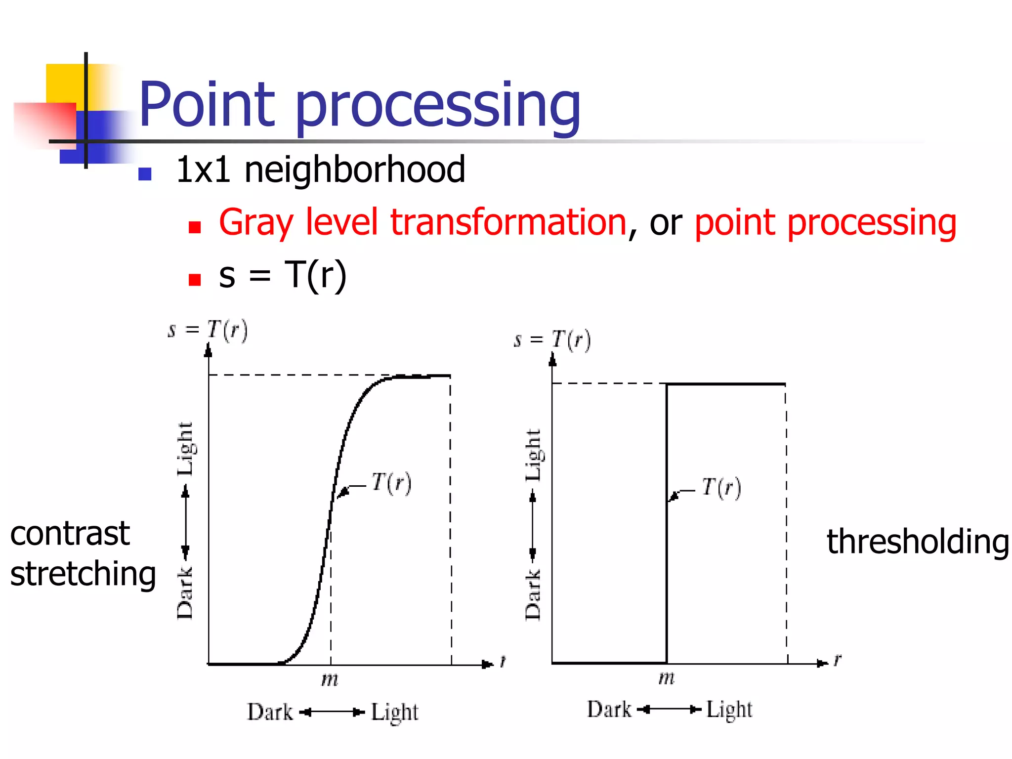
 Spatial domain processing
 g(x,y)=T[ f(x,y) ]
 f(x,y): input image
 g(x,y): output image
 T: operator
 Defined over some neighborhood of (x,y)
T
f(x,y) g(x,y)

7. Background (cont.)
* T operates over
neighborhood of (x,y)
* T applies to each pixel
in the input image

8. Point processing
 1x1 neighborhood
 Gray level transformation, or point processing
 s = T(r)
contrast
stretching
thresholding

9. 9
Image Enhancement by Point
Processing
 Contrast Stretching

10. Bahadir K. Gunturk 10
Image Enhancement by Point
Processing
 Contrast Stretching
( ) log(1 )
T r c r
 

11. Neighborhood processing
 A larger predefined neighborhood
 Ex. 3x3 neighborhood
 mask, filters, kernels, templates, windows
 Mask processing or filtering

12. Some Basic Gray Level Transformations
 Image negatives (complement)
 Log transformation
 Power-law transform
 Piece-wise linear transform
 Gray level slicing
 Bit plane slicing

13. Some gray level transformations
•Lookup table
•Functional form

14. Image negatives
 Photographic negative 負片
 Suitable for images with dominant black
areas
Original mammogram(乳房X光片)

15. Log transformations
 s = c log(1+r)
 Compress the dynamic
range of images with
large variation in pixel
values

16. Example: Log transformations
 log(fft2(I)) : log of Fourier transform
2d Fourier transform 頻譜圖
log

17. Power-law transformations
 s=cr
 >1
 <1
 : gamma
 display, printers,
scanners follow
power-law
 Gamma correction

18. Example: Gamma correction
 CRT: intensity-to-
voltage response
follow a power-law.
1.8<<2.5
=2.5
=1/2.5
=2.5
原始影像 顯示器偏差

19. Power-law:
 Expand dark gray
levels
<1
=0.6
=0.3
=0.4

20. Power-law: >1
 Expand light
gray levels
=4 =5
=3

21. Piece-wise linear transformations
 Advantage: the
piecewise function
can be arbitrarily
complex
control point

22. Contrast
stretching
How to automatically adjust
the gray levels?

23. Gray-level slicing 切片
 Highlighting a specific range of gray levels

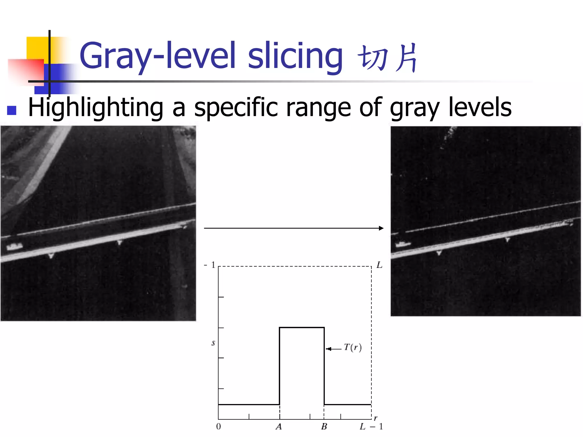
24. Gray-level slicing
 Highlighting a specific
range of gray levels in an
image
 Display a high value of all
gray levels in the range of
interest and a low value for
all other gray levels
 (a) transformation highlights
range [A,B] of gray level and
reduces all others to a
constant level
 (b) transformation highlights
range [A,B] but preserves all
other levels

25. Bit-plane slicing
* Highlight specific bits
bit-planes of an image
(gray level 0~255)
Ex. 15010
1
0
0
1
0
1
0
0

26. Bit-plane slicing: example

27. 7 6
5 4 3
2 1 0
For image
compression

28. Arithmetic/logic operations
 Logic operations
 Image subtraction
 Image averaging

29. Logic operations
 Logic operations: pixel-wise AND, OR, NOT
 The pixel gray level values are taken as
string of binary numbers
 Use the binary mask to take out the region
of interest(ROI) from an image
Ex. 193 => 11000001

30. Logic operations: example
AND
OR
A B A and B
A or B

31. Image subtraction
 Difference image
g(x,y)=f(x,y)-h(x,y)
f:original(8 bits) h:4 sig. bits
difference image
scaling

32. Image subtraction: scaling the
difference image
 g(x,y)=f(x,y)-h(x,y)
 f and h are 8-bit => g(x,y)  [-255, 255]
1. (1)+255 (2) divide by 2
• The result won’t cover [0,255]
2. (1)-min(g) (2) *255/max(g)
Be careful of the dynamic range after the image
is processed.

33. Image subtraction example:
mask mode radiography
 Inject contrast medium into bloodstream
original (head) difference image
注射碘液
拍攝影像
與原影像
相減

34. Image averaging
 Noisy image g(x,y)=f(x,y)+η(x,y)
 Suppose η(x,y) is uncorrelated and has zero
mean
original noise
Clear image Noisy image

35. Image averaging: noise
reduction
  )
,
(
)
,
( y
x
f
y
x
g
E 
2
)
,
(
2
)
,
(
1
y
x
y
x
g
K


 
期望值接近原圖

 2

K
 Averaging over K noisy images gi(x,y)



K
i
i y
x
g
K
y
x
g
1
)
,
(
1
)
,
(

36. original Gaussian
noise
averaging
K=8
averaging
K=16
averaging
K=64
averaging
K=128