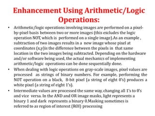
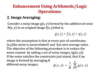
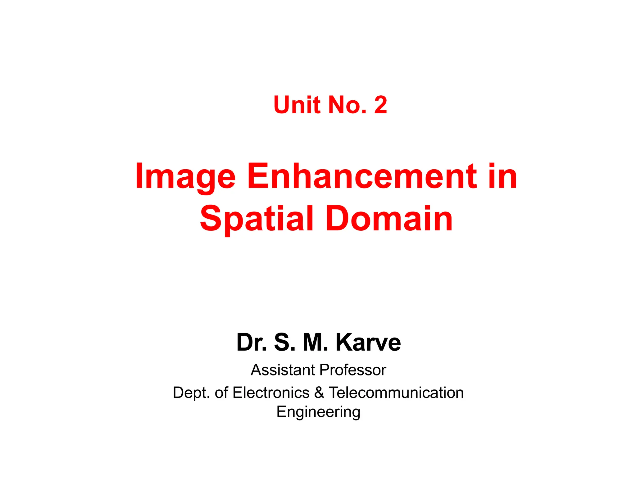
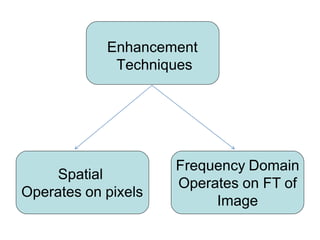
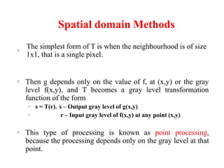
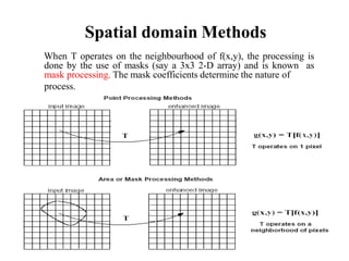
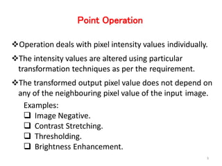
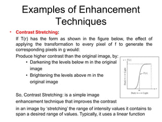
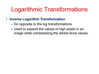
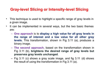
The document discusses various image enhancement techniques in the spatial domain. It describes point processing and mask processing as two types of spatial domain methods. Point processing involves transformations based on individual pixel intensities, while mask processing uses neighborhoods of pixels. Examples of point processing techniques include contrast stretching, thresholding, and logarithmic, power-law, and piecewise linear transformations. Histogram processing and arithmetic/logic operations are also discussed as methods for image enhancement in the spatial domain.

1. Unit No. 2
Image Enhancement in
Spatial Domain
Dr. S. M. Karve
Assistant Professor
Dept. of Electronics & Telecommunication
Engineering

2. Image Enhancement Definition
• Image Enhancement: is the process that
improves the quality of the image for a
specific application

3. Image Enhancement Methods
• Spatial Domain Methods (Image Plane)
Techniques are based on direct manipulation of
pixels in an image
• Frequency Domain Methods
Techniques are based on modifying the
Fourier transform of the image.
• Combination Methods
There are some enhancement techniques
based on various combinations of methods
from the first two categories

4. Enhancement
Techniques
Spatial
Operates on pixels
Frequency Domain
Operates on FT of
Image

5. Spatial domain Methods

The simplest form of T is when the neighbourhood is of size
1x1, that is a single pixel.
 Then g depends only on the value of f, at (x,y) or the gray
level f(x,y), and T becomes a gray level transformation
function of the form
 s = T(r). s – Output gray level of g(x,y)
r – Input gray level of f(x,y) at any point (x,y)

 This type of processing is known as point processing,
because the processing depends only on the gray level at that
point.

6. When T operates on the neighbourhood of f(x,y), the processing is
done by the use of masks (say a 3x3 2-D array) and is known as
mask processing. The mask coefficients determine the nature of
process.
Spatial domain Methods

7. Point Operation
Operation deals with pixel intensity values individually.
The intensity values are altered using particular
transformation techniques as per the requirement.
The transformed output pixel value does not depend on
any of the neighbouring pixel value of the input image.
Examples:
 Image Negative.
 Contrast Stretching.
 Thresholding.
 Brightness Enhancement.
3

8. Examples of Enhancement
Techniques
• Contrast Stretching:
If T(r) has the form as shown in the figure below, the effect of
applying the transformation to every pixel of f to generate the
corresponding pixels in g would:
Produce higher contrast than the original image, by:
• Darkening the levels below m in the original
image
• Brightening the levels above m in the
original image
So, Contrast Stretching: is a simple image
enhancement technique that improves the contrast
in an image by ‘stretching’ the range of intensity values it contains to
span a desired range of values. Typically, it uses a linear function

9. Examples of Enhancement
Techniques
• Thresholding
Is a limited case of contrast stretching, it produces a two-level
(binary) image.
Some fairly simple, yet powerful, processing approaches can be
formulated with grey-level transformations. Because enhancement
at any point in an image depends only on the gray level at that point,
techniques in this category often are referred to as point processing.

10. Basic Intensity (Gray-level)
Transformation Functions
• Grey-level transformation functions (also called,
intensity functions), are considered the simplest of all
image enhancement techniques.
The value of pixels, before and after processing, will
be denoted by r and s, respectively.
These values are related by the expression of the
form:
s = T (r)
where T is a transformation that maps a pixel value r
into a pixel value s.
•
•

11. Consider the following figure, which shows three basic types of
functions used frequently for image enhancement:
Basic Intensity (Gray-level)
Transformation Functions

12. Basic Intensity (Gray-level)
Transformation Functions
• The three basic types of functions used frequently for
image enhancement:
– Linear Functions:
• Negative Transformation
• Identity Transformation
– Logarithmic Functions:
• Log Transformation
• Inverse-log Transformation
– Power-Law Functions:
• nthpower transformation
• nthroot transformation

13. Linear Functions
• Identity Function
– Output intensities are identical to input
intensities
– This function doesn’t have an effect on an
image, it was included in the graph only for
completeness
– Its expression:
s = r

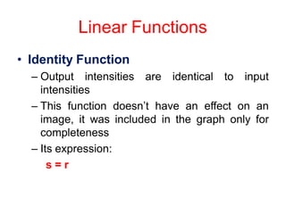
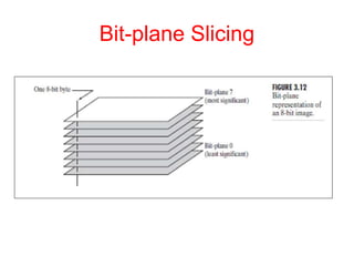
14. Linear Functions
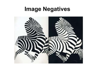
• Image Negatives (Negative Transformation)
– The negative of an image with gray level in the range [0, L-1],
where L = Largest value in an image, is obtained by using the
negative transformation’s expression:
s = L – 1 – r
Which reverses the intensity levels of an input image, in this
manner produces the equivalent of a photographic negative.
– The negative transformation is suitable for enhancing white
or gray detail embedded in dark regions of an image,
especially when the black area are dominant in size

15. Image Negatives

16. Logarithmic Transformations
• Log Transformation
The general form of the log transformation:
s = c log (1+r)
Where c is a constant, and r ≥ 0
– Log curve maps a narrow range of low gray-level values
in the input image into a wider range of the output levels.
– Used to expand the values of dark pixels in an image
while compressing the higher-level values.
– It compresses the dynamic range of images with large
variations in pixel values.

17. Logarithmic Transformations

18. Logarithmic Transformations
• Inverse Logarithm Transformation
– Do opposite to the log transformations
– Used to expand the values of high pixels in an
image while compressing the darker-level values.

19. Power-Law Transformations
• Power-law transformations have the basic
form of:
s = c . rᵞ
Where c and ᵞ are positive constants

20. Power-Law Transformations
• Different transformation curves are obtained
by varying ᵞ (gamma)

21. Power-Law Transformations
• Variety of devices used for image capture, printing and display respond
according to a power law. The process used to correct this power-law
response phenomena is called gamma correction.
For example, Cathode Ray Tube (CRT) devices have an intensity-to-
voltage response that is a power function, with exponents varying
from approximately 1.8 to 2.5.With reference to the curve for g=2.5 in Fig.
3.6, we see that such display systems would tend to produce images
that are darker than intended. This effect is illustrated in Fig. 3.7. Figure
3.7(a) shows a simple gray-scale linear wedge input into a CRT monitor. As
expected, the output of the monitor appears darker than the input, as shown
in Fig. 3.7(b). Gamma correction. In this case is straightforward. All we
need to do is preprocess the input image before inputting it into the
monitor by performing the transformation. The result is shown in Fig.
3.7(c).When input into the same monitor, this gamma-corrected input
produces an output that is close in appearance to the original image, as
shown in Fig. 3.7(d).

22. Power-Law Transformation

23. Power-Law Transformation
• In addition to
gamma
correction,
power-law
transformations
are useful for
general-
purpose
contrast
manipulation.
See figure 3.8

24. Power-Law Transformation
• Another
illustration of
Power-law
transformation

25. Piecewise-Linear Transformation
Functions
• Principle: Rather than using a well defined
mathematical function we can use arbitrary
user defined transforms
• Advantage: Some important transformations
can be formulated only as a piecewise function.
• Disadvantage: Their specification requires more
user input that previous transformations

26. Types of Piecewise transformations
– Contrast Stretching
– Gray-level Slicing
– Bit-plane slicing

27. Contrast Stretching
• One of
functions
the simplest piecewise linear
is a contrast-stretching
transformation, which is used to enhance
the low contrast images.
• Low contrast images may result from:
– Poor illumination
– Wrong setting of lens aperture during image
acquisition.

28. Contrast Stretching

29. Contrast Stretching
• Figure 3.10(a) shows a typical transformation used for contrast
stretching.
The locations of points (r1, s1) and (r2, s2) control the shape of the
transformation function.
If r1 = s1 and r2 = s2, the transformation is a linear function that
produces no changes in gray levels.
If r1 = r2, s1 = 0 and s2 = L-1, the transformation becomes a
Thresholding function that creates a binary image.
Intermediate values of (r1, s1) and (r2, s2) produce various
degrees of spread in the gray levels of the output image, thus
affecting its contrast.
In general, r1 ≤ r2 and s1 ≤ s2 is assumed, so the function is
always increasing.
•
•
•
•
•

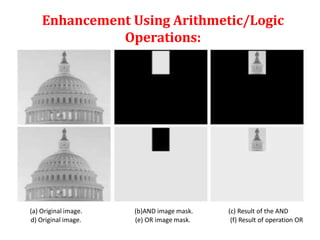
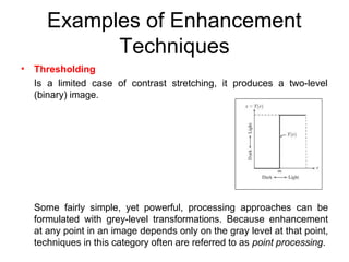
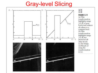
30. Contrast Stretching
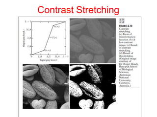
• Figure 3.10(b) shows an 8-bit image with low contrast.
• Fig. 3.10(c) shows the result of contrast stretching, obtained by
setting (r1, s1) = (rmin, 0) and (r2, s2) = (rmax,L-1) where rminand rma
x
denote the minimum and maximum gray levels in the image,
respectively. Thus, the transformation function stretched the levels
linearly from their original range to the full range [0, L-1].
• Finally, Fig. 3.10(d) shows the result of using the thresholding
function defined previously, with r1=r2=m, the mean gray level in the
image.

31. Gray-level Slicing or Intensity-level Slicing
• This technique is used to highlight a specific range of gray levels in
a given image.
It can be implemented in several ways, but the two basic themes
are:
– One approach is to display a high value for all gray levels in
the range of interest and a low value for all other gray
levels. This transformation, shown in Fig 3.11 (a), produces a
binary image.
– The second approach, based on the transformation shown in
Fig 3.11 (b), brightens the desired range of gray levels but
preserves gray levels unchanged.
– Fig 3.11 (c) shows a gray scale image, and fig 3.11 (d) shows
the result of using the transformation in Fig 3.11 (a).
•

32. Gray-level Slicing

33. Bit-plane Slicing
•
•
Pixels are digital numbers, each one composed of bits.
For example, the intensity of each pixel in a 256 gray –
scale image is composed of 8 bits (ie 1 byte)
• Instead of highlighting gray-level range, we could
highlight the contribution made by each bit.
This method is useful and used in image compression.
•

34. Bit-plane Slicing

35. Bit-plane Slicing
• Assuming that each pixel is represented by 8 bits, the
image is composed of eight 1-bit planes
Plane 0 containing the lowest order bit of all pixels in the
image and plane 7 all the higher order bits
Only the most significant bits contain the majority of
visually significant data. The other bit planes constitute
the most suitable details
Separating a digital image into its bits planes is useful for
analyzing the relative importance played by each bit of
the image
It helps in determining the adequacy of the number of
bits used to quantize each pixel
•
•
•
•

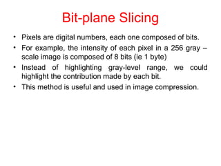
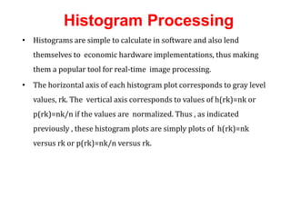
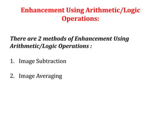
36. Histogram Processing
• Histograms are the basis for numerous spatial domain processing
techniques. Histogram manipulation can be used effectively for
image enhancement.
• The histogram of a digital image with gray levels in the range [0,L-1] is a
discrete function h(rk)=nk, where rk is the kth gray level and nk is the
number of pixels in the image having gray level rk. It is common
practice to normalize a histogram by dividing each of its values by the
total number of pixels in the image, denoted by n.Thus, a normalized
histogram is given by p(rk)=nk/n, for k=0,1,p,L-1.Loosely speaking,
p(rk) gives an estimate of the probability of occurrence of gray level rk.
Note that the sum of all components of a normalized histogram is equal
to 1. (negative and identity transformations)

37. Histogram Processing
• Histograms are simple to calculate in software and also lend
themselves to economic hardware implementations, thus making
them a popular tool for real-time image processing.
• The horizontal axis of each histogram plot corresponds to gray level
values, rk. The vertical axis corresponds to values of h(rk)=nk or
p(rk)=nk/n if the values are normalized. Thus , as indicated
previously , these histogram plots are simply plots of h(rk)=nk
versus rk or p(rk)=nk/n versus rk.

38. Histogram Processing
Fig: Four basic image types : dark, light , low contrast, high contrast
,and their corresponding histograms.

39. Histogram Processing
(a)OriginalImage (b)Negative Transformation
1. Histogram Equalization:
It is a technique for adjusting image
intensities to enhance contrast. Let f be a
given image represented as a mr by mc
matrix of integer pixel intensities
ranging. So L is the number of possible
intensity values, often 256. Let p denote
the normalized histogram of f with a bin
for each possible intensity. So
Pn = number of pixels with intensity
n /total number of pixels
Where n = 0,1,...,L − 1.

40. Histogram Processing
2. Histogram Matching (Specification):
In image processing, histogram matching or histogram specification is
the transformation of an image so that its histogram matches a specified
histogram.
When automatic enhancement is desired, this is a good approach because
the results from this technique are predictable and the method is simple
to implement. In particular, it is useful sometimes to be able to specify the
shape of the histogram that we wish the processed image to have. The
method used to generate a processed image that has a specified histogram
is called histogram matching or histogram specification.
Here we want to convert the image so that it has a particular histogram
that can be arbitrarily specified. Such a mapping function can
be found in three steps:
• Equalize the histogram of the input image
• Equalize the specified histogram
• Relate the two equalized histograms

41. Histogram Processing
We first equalize the histogram Px of the
input image x :
We then equalize the desired histogramPz of the
output image z :
The inverse of the above transform is
As the two intermediate images Y andY’ both have the same equalized histogram, they
are actually the same image, i.e., Y=Y’ , and the overall transform from the given
image x to the desired image z can be found to be:
2. Histogram Matching (Specification):

42. Enhancement Using Arithmetic/Logic
Operations:
• Arithmetic/logic operations involving images are performed on a pixel-
by-pixel basis between two or more images (this excludes the logic
operation NOT, which is performed on a single image).As an example ,
subtraction of two images results in a new image whose pixel at
coordinates (x,y)is the difference between the pixels in that same
location in the two images being subtracted. Depending on the hardware
and/or software being used, the actual mechanics of implementing
arithmetic/logic operations can be done sequentially done.
• When dealing with logic operations on gray-scale images, pixel values are
processed as strings of binary numbers. For example, performing the
NOT operation on a black, 8-bit pixel (a string of eight 0’s) produces a
white pixel (a string of eight 1’s).
• Intermediate values are processed the same way, changing all 1’s to 0’s
and vice versa. In the AND and OR image masks, light represents a
binary 1 and dark represents a binary 0.Masking sometimes is
referred to as region of interest (ROI) processing

43. Enhancement Using Arithmetic/Logic
Operations:
(a) Original image. (b)AND image mask. (c) Result of the AND
d) Original image. (e) OR image mask. (f) Result of operation OR

44. Enhancement Using Arithmetic/Logic
Operations:
There are 2 methods of Enhancement Using
Arithmetic/Logic Operations :
1. Image Subtraction
2. Image Averaging

45. Enhancement Using Arithmetic/Logic
Operations:
1. Image Subtraction:
Image subtraction or pixel subtraction is a process whereby the
digital numeric value of one pixel or whole image is subtracted from
another image. This is primarily done for one of two reasons – levelling
uneven sections of an image such as half an image having a shadow on it,
or detecting changes between two images.This detection of changes can
be used to tell if something in the image moved. This is commonly used
in fields such as astrophotography to assist with the computerized
search for asteroids in which the target is moving and would be in one
place in one image, and another from an image one hour later and
where using this technique would make the fixed stars in the
background disappear leaving only the target.
The difference between two images f(x, y) and h(x, y), expressed as

46. Enhancement Using Arithmetic/Logic
Operations:
2. Image Averaging:
Consider a noisy image g(x, y) formed by the addition of noise
N(x, y) to an original image f(x, y);that is,
where the assumption is that at every pair of coordinates
(x,y)the noise is uncorrelated† and has zero average value.
The objective of the following procedure is to reduce the
noise content by adding a set of noisy images, {gi(x, y)}
If the noise satisfies the constraints just stated, that if an
image is formed by averaging K
different noisy images,