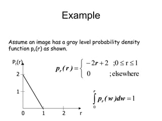
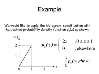
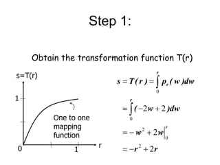
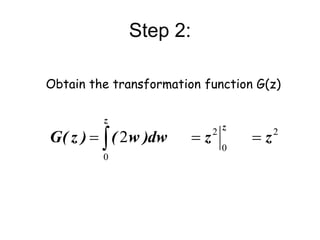
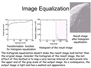
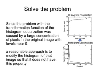
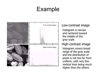
This document discusses various techniques for enhancing images in the spatial domain, which involves direct manipulation of pixel values. It describes point processing techniques like gray-level transformations that map input pixel values to output values using functions like negative, logarithm, power-law, and piecewise linear. Histogram processing techniques are also covered, including histogram equalization, which spreads out the most frequent intensity values in an image. The document provides examples to illustrate the effect of these different enhancement methods.


![Spatial Domain
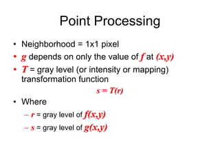
• Procedures that operate
directly on pixels.
g(x,y) = T[f(x,y)]
where
– f(x,y) is the input image
– g(x,y) is the processed
image
– T is an operator on f
defined over some
neighborhood of (x,y)](https://image.slidesharecdn.com/imageenhancementinthespatialdomain1-240302102330-a2132f4c/85/Image-Enhancement-in-the-Spatial-Domain1-ppt-5-320.jpg)
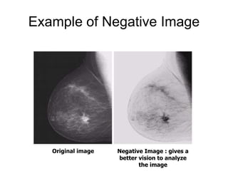
![Image Negatives
• An image with gray level in the
range [0, L-1]
where L = 2n ; n = 1, 2…
• Negative transformation :
s = L – 1 –r
• Reversing the intensity levels
of an image.
• Suitable for enhancing white
or gray detail embedded in
dark regions of an image,
especially when the black area
dominant in size.
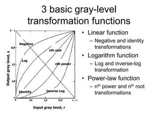
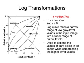
Input gray level, r
Negative
Log
nth root
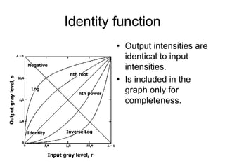
Identity
nth power
Inverse Log](https://image.slidesharecdn.com/imageenhancementinthespatialdomain1-240302102330-a2132f4c/85/Image-Enhancement-in-the-Spatial-Domain1-ppt-9-320.jpg)


![Gray-level slicing
• Highlighting a specific
range of gray levels in an
image
– Display a high value of all
gray levels in the range of
interest and a low value for
all other gray levels
• (a) transformation highlights
range [A,B] of gray level and
reduces all others to a
constant level
• (b) transformation highlights
range [A,B] but preserves all
other levels](https://image.slidesharecdn.com/imageenhancementinthespatialdomain1-240302102330-a2132f4c/85/Image-Enhancement-in-the-Spatial-Domain1-ppt-22-320.jpg)

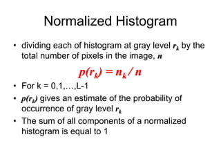
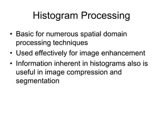
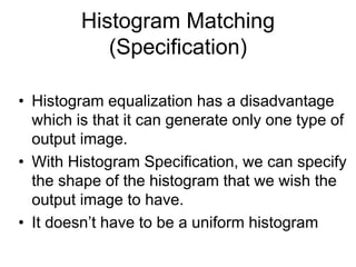
![Histogram Processing
• Histogram of a digital image with gray levels in
the range [0,L-1] is a discrete function
h(rk) = nk
• Where
– rk : the kth gray level
– nk : the number of pixels in the image having gray
level rk
– h(rk) : histogram of a digital image with gray levels rk](https://image.slidesharecdn.com/imageenhancementinthespatialdomain1-240302102330-a2132f4c/85/Image-Enhancement-in-the-Spatial-Domain1-ppt-26-320.jpg)
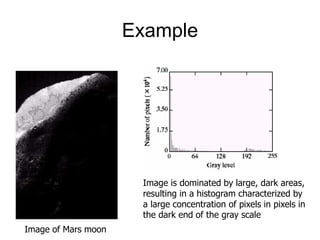
![Example
2 3 3 2
4 2 4 3
3 2 3 5
2 4 2 4
4x4 image
Gray scale = [0,9]
histogram
0 1
1
2
2
3
3
4
4
5
5
6
6
7 8 9
No. of pixels
Gray level](https://image.slidesharecdn.com/imageenhancementinthespatialdomain1-240302102330-a2132f4c/85/Image-Enhancement-in-the-Spatial-Domain1-ppt-27-320.jpg)
![Example
2 3 3 2
4 2 4 3
3 2 3 5
2 4 2 4
4x4 image
Gray scale = [0,9]
histogram
0 1
1
2
2
3
3
4
4
5
5
6
6
7 8 9
No. of pixels
Gray level](https://image.slidesharecdn.com/imageenhancementinthespatialdomain1-240302102330-a2132f4c/85/Image-Enhancement-in-the-Spatial-Domain1-ppt-35-320.jpg)
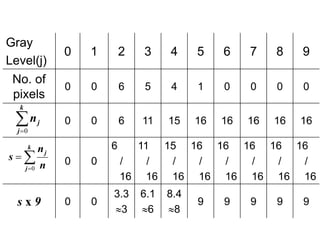
![Example
3 6 6 3
8 3 8 6
6 3 6 9
3 8 3 8
Output image
Gray scale = [0,9]
Histogram equalization
0 1
1
2
2
3
3
4
4
5
5
6
6
7 8 9
No. of pixels
Gray level](https://image.slidesharecdn.com/imageenhancementinthespatialdomain1-240302102330-a2132f4c/85/Image-Enhancement-in-the-Spatial-Domain1-ppt-37-320.jpg)
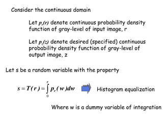
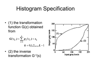
![Next, we define a random variable z with the property
s = T(r) = G(z)
We can map an input gray level r to output gray level z
thus
s
dt
)
t
(
p
)
z
(
g
z
z
0
Where t is a dummy variable of integration
Histogram equalization
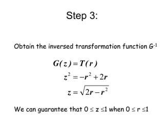
Therefore, z must satisfy the condition
z = G-1(s) = G-1[T(r)]
Assume G-1 exists and satisfies the condition (a) and (b)](https://image.slidesharecdn.com/imageenhancementinthespatialdomain1-240302102330-a2132f4c/85/Image-Enhancement-in-the-Spatial-Domain1-ppt-40-320.jpg)
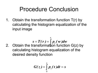
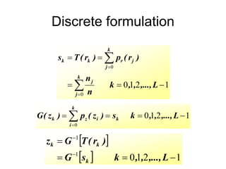
![Procedure Conclusion
3. Obtain the inversed transformation
function G-1
4. Obtain the output image by applying the
processed gray-level from the inversed
transformation function to all the pixels in
the input image
z = G-1(s) = G-1[T(r)]](https://image.slidesharecdn.com/imageenhancementinthespatialdomain1-240302102330-a2132f4c/85/Image-Enhancement-in-the-Spatial-Domain1-ppt-42-320.jpg)