Digital Image Processing - Image Enhancement (NOTES) Material or Tips for Engineering students ...................

1. Unit III Image Enhancement
Two mark Questions with Answers
1. What is a mask?
A Mask is a small two-dimensional array, in which the value of
the mask coefficient determines the nature of the process, such as image
sharpening.
The enhancement technique based on this type of approach is
referred to as mask processing.
2. How can an image negative be obtained?
The negative of an image with gray levels in the range [0, L-1] is obtained
by using the negative transformation, which is given by the expression.
s = L-1- r, where„s‟ is output pixel, „r‟ is input pixel
3. What is the difference between contrast stretching and compression of
dynamic range?
Contrast Stretching
Produce higher contrast than the original by
 Darkening the levels below m in the original image.
 Brightening the levels above m in the original image.
Compression of dynamic range
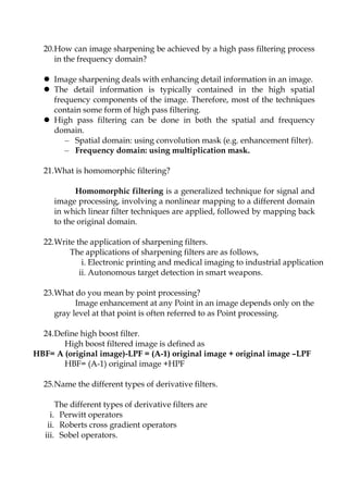
 It compresses the dynamic range of images with large
variations in pixel values
 Example of image with dynamic range: Fourier spectrum
image
 It can have intensity range from 0 to 106 or higher.
 We can‟t see the significant degree of detail as it will be lost
in the display.
The contrast stretching increases the dynamic range of the gray
levels

2. 4. What is a histogram?
Histogram of a digital image with gray levels in the range [0,L-1] is
a discrete function.
h(rk) = nk
Where,
rk : the kth gray level
nk : the number of pixels in the image having gray level rk
h(rk) : histogram of a digital image with gray levels rk
5. What is meant by histogram equalization?
It is a technique used to obtain linear histogram. It is also known
as histogram linearization. Condition for uniform histogram is
Ps(s) = 1
(or)
The histogram equalization is an approach to enhance a given
image. The approach is to design a transformation T(.) such that the
gray values in the output is uniformly distributed in [0, 1].
6. How can histogram equalization be applied locally?
 Histogram processing methods are global processing, in the sense
that pixels are modified by a transformation function based on
the gray-level content of an entire image.
 Sometimes, we may need to enhance details over small areas in
an image, which is called a local enhancement.
7. What is Image Enhancement?
Image enhancement is a technique to process an image so that the
result is more suitable than the original image for specific applications.
8. In local Histogram processing, why are non-overlapping regions used?
It‟s used to reduce computation is to utilize nonoverlapping
regions, but it usually produces an undesirable checkerboard effect.

3. 9. What is meant by histogram matching or histogram specification?
Histogram equalization yields an image whose pixels are (in
theory) uniformly distributed among all gray levels. Sometimes, this
may not be desirable. Instead, we may want a transformation that
yields an output image with a pre-specified histogram. This technique
is called histogram specification.
10.How can noise reduction be accomplished using image averaging?
Consider a noisy image g(x,y) formed by the addition of noise (x,y) to
an original image f(x,y).
g(x,y) = f(x,y) + (x,y)
 if noise has zero mean and be uncorrelated then it can be shown that if
),( yxg
Then,
),(
2
),(
2
, yxyxg 
if „K‟ increase, it indicates that the variability (noise) of the pixel at each
location (x,y) decreases.
11.Differentiate between linear and nonlinear spatial filters.
s.no. Linear spatial filter Non-linear spatial filter
1.
2.
Response is a sum of
products of the filter co-
efficient.
R = w(-1,-1) f(x-1,y-1) +
w(-1,0) f(x-1,y) + … +
w(0,0) f(x,y) + … +
w(1,0) f(x+1,y) +
w(1,1) f(x+1,y+1).
They do not explicitly use co-
efficients in the sum-of-
products.
R = w1z1 + w2z2 + … +w9z9
9
= ∑ wizi
i=1
1
( , ) ( , )
1
K
g x y g x yiK i
 

12 2
( , ) ( , )g x y x yK
 



4. 12.What is image Negatives?
The negative of an image with gray levels in the range [0, L-1] is
obtained by using the negative transformation, which is given by the
expression.
s = L-1- r, Where s is output pixel, r is input pixel
13.Differentiate between Correlation and Convolution with specific
reference to an image and a filter mask.
Convolution in frequency domain reduces the multiplication in the x
domain
The correlation of 2 continuous functions f(x) and g(x) is defined by
14.Define derivative filter.
For a function f (x, y), the gradient f at co-ordinate (x, y) is defined as
the vector
15.What is the principal difficulty with the smoothing method with
reference to edges and sharp details?
 Median filtering is a powerful smoothing technique that does not blur
the edges significantly .
 Max/min filtering is used where the max or min value of the
neighbourhood gray levels replaces the candidatepel .

5.  Shrinking and expansion are useful operations especially in two tone
images.
16.What is the basic characteristic of a high pass filter mask coefficients?
 The basic strategy behind weighting the center point the highest and
then reducing the value of the coefficients as a function of increasing
distance from the origin is simply an attempt to reduce blurring in the
smoothing process.
17.What is the effect of averaging with reference to detail in an image?
An important application of image averaging is in the field of
astronomy, where imaging with very low light levels is routine, causing
sensor noise frequently to render single images virtually useless for
analysis.
18.Outline a simple procedure to produce an enhanced image using a
fourier transform and a filter transfer function.
Frequency domain techniques are based on modifying the Fourier
transform of an image.
19.How can blurring or smoothing process be explained in the frequency
domain?
Smoothing Filters are used for blurring and for noise reduction
�Blurring is used for removal of small details prior to object
extraction.
�bridging of small gaps in lines or curves.
�Smoothing Linear Filters (Averaging Filters)
�replace the average value defined by the filter mask.
�have the undesirable effect of blur edges

6. 20.How can image sharpening be achieved by a high pass filtering process
in the frequency domain?
 Image sharpening deals with enhancing detail information in an image.
 The detail information is typically contained in the high spatial
frequency components of the image. Therefore, most of the techniques
contain some form of high pass filtering.
 High pass filtering can be done in both the spatial and frequency
domain.
– Spatial domain: using convolution mask (e.g. enhancement filter).
– Frequency domain: using multiplication mask.
21.What is homomorphic filtering?
Homomorphic filtering is a generalized technique for signal and
image processing, involving a nonlinear mapping to a different domain
in which linear filter techniques are applied, followed by mapping back
to the original domain.
22.Write the application of sharpening filters.
The applications of sharpening filters are as follows,
i. Electronic printing and medical imaging to industrial application
ii. Autonomous target detection in smart weapons.
23.What do you mean by point processing?
Image enhancement at any Point in an image depends only on the
gray level at that point is often referred to as Point processing.
24.Define high boost filter.
High boost filtered image is defined as
HBF= A (original image)-LPF = (A-1) original image + original image –LPF
HBF= (A-1) original image +HPF
25.Name the different types of derivative filters.
The different types of derivative filters are
i. Perwitt operators
ii. Roberts cross gradient operators
iii. Sobel operators.

7. Twelve mark Questions
1. What is image enhancement? Explain Contrast stretching and
compression of dynamic range.
Image enhancement is a technique to process an image so that the
result is more suitable than the original image for specific
applications.
 The suitableness is up to each application.
 A method which is quite useful for enhancing an image may
not necessarily be the best approach for enhancing another
images
 Image enhancement widely used in computer graphics.
 It is the sub areas of image processing.
Enhancement approaches:
1. Spatial domain 2. Frequency domain
1) Spatial Domain : (image plane)
 Techniques are based on direct manipulation of pixels in an
image.
2) Frequency Domain :
 Techniques are based on modifying the Fourier transform of an
image.
There are some enhancement techniques based on various
combinations of methods from these two categories.
Contrast Stretching
Low contrast images occur often due to poor or nonuniform
lighting conditions or due to nonlinearity or small dynamic range of the
image sensor.
Expands the range of intensity levels in an image so that it spans
the full intensity range of the recording medium or display device.

8. The figure shows a typical contrast stretching transformation
FIG : Contrast Stretching Transformation
For , Dark region stretch 1,
3
L
a  ;
Mid region stretch
2
1,
3
L
b  ;
Bright region stretch 1 
Which can be expressed as,
, 0
( ) ,
( ) ,
a
b
u for u a
u a V for a u b
u b V for b u L

 

  

     
     
The slope of the transformation is chosen greater than unity in the
region of stretch.
The parameters a & b can be obtained by examining the histogram of
the image.
For example, the gray scale intervals where pixels occur most
frequently would be stretched most to improve the overall visibility of
the scene.
Produce Higher contrast than the original image:
 By darkening the levels below „m‟ in the original image.
 By Brightening the levels above „m‟ in the original image.

9. Compression of dynamic range.
Sometimes the dynamic range of the image data may be very large.
For example, the dynamic range of a typical unitarily transformed
image is so large that only a few pixels are visible.
The dynamic range can be compressed via the logarithmic
transformation.
log (1 )
10
C u  
Where „C‟ is a scaling constant and „u‟ is a Gray levels.
This transformation enhance the small magnitude pixels compared to
those pixels with large magnitudes.

10. 2. Explain histogram equalization and histogram specification. How can
they be applied for local enhancement?
Histogram Processing
Histogram of a digital image with gray levels in the range [0,L-1] is a
discrete function
h(rk) = nk
Where
rk : the kth gray level
nk : the number of pixels in the image having gray
level rk
h(rk) : histogram of a digital image with gray levels rk
Histogram Equalization
Histogram EQUALization
Aim: To “equalize” the histogram, to “flatten”, “distrubute as uniform
as possible”.
● As the low-contrast image's histogram is narrow and centred towards
the middle of the gray scale, by distributing the histogram to a wider
range will improve the quality of the image.
● Adjust probability density function of the original histogram so that the
probabilities spread equally
The histogram equalization is an approach to enhance a given image.
The approach is to design a transformation T(.) such that the gray
values in the output is uniformly distributed in [0, 1].
Let us assume for the moment that the input image to be enhanced
has continuous gray values, with r = 0 representing black and r = 1
representing white.
We need to design a gray value transformation s = T(r), based on the
histogram of the input image, which will enhance the image.

11. As before, we assume that:
(1) T(r) is a monotonically increasing function for 0≤r≤1 (preserves
order from black to white).
(2) T(r) maps [0,1] into [0,1] (preserves the range of allowed Gray
values).
Let us denote the inverse transformation by r = T -1(s) . We assume that
the inverse transformation also satisfies the above two conditions.
We consider the gray values in the input image and output image as
random variables in the interval [0, 1].
Let pin(r) and pout(s) denote the probability density of the Gray values in
the input and output images.
If pin(r) and T(r) are known, and r = T -1(s) satisfies condition 1, we can
write (result from probability theory):
( ) ( )
1( )
dr
p s p rout in ds r T s
 
 
 


One way to enhance the image is to design a transformation T(.) such
that the gray values in the output is uniformly distributed in [0, 1], i.e.
pout (s) = 1, 0≤s≤1 .
In terms of histograms, the output image will have all gray values in
“equal proportion”. This technique is called histogram equalization.

12. Next we derive the gray values in the output is uniformly distributed in
[0, 1].
·Consider the transformation
( ) ( ) 0 1,0
rs T r p w dw r
in
   
Note that this is the cumulative distribution function (CDF) of pin (r)
and satisfies the previous two conditions.
From the previous equation and using the fundamental theorem of
calculus,
( )ds p r
indr

Therefore, the output histogram is given by
1( ) ( ) 1 1, 0 11( )( ) 1( )
p s p r sr T sout in p r
in r T s
 
   
   
  
     

The output probability density function is uniform, regardless of the
input.
Thus, using a transformation function equal to the CDF of input gray
values r, we can obtain an image with uniform gray values.
This usually results in an enhanced image, with an increase in the
dynamic range of pixel values.
How to implement histogram equalization?
Step 1:For images with discrete gray values, compute:
( )
n
kp r
in nk
 0 1r
k
  0 1k L  
L: Total number of gray levels
nk: Number of pixels with gray value rk

13. n: Total number of pixels in the image
Step 2: Based on CDF, compute the discrete version of the previous
transformation :
( ) ( )
0
k
s T r p r
in jk k j
  

0 1k L  
Example:
Consider an 8-level 64 x 64 image with gray values (0, 1, …,7). The
normalized gray values are (0, 1/7, 2/7, …, 1). The normalized
histogram is given below:
NB: The gray values in output are also (0, 1/7, 2/7, …, 1).
Notice that there are only five distinct gray levels --- (1/7, 3/7,5/7, 6/7,
1) in the output image. We will relabel them as (s0,s1, …, s4 ).
With this transformation, the output image will have histogram

14. Histogram Specification (Histogram Matching)
Histogram equalization yields an image whose pixels are (in theory)
uniformly distributed among all gray levels.
Sometimes, this may not be desirable. Instead, we may want a
transformation that yields an output image with a pre-specified
histogram. This technique is called histogram specification.
 Given Information
(1) Input image from which we can compute its histogram .
(2) Desired histogram.
 Goal
Derive a point operation, H(r), that maps the input image into
an output image that has the user-specified histogram.
Again, we will assume, for the moment, continuous-gray values.
Approach of derivation
Step1: Equalize the levels of the original image
Step2: Specify the desired pdf and obtain the transformation function
Step3: Apply the inverse transformation function to the levels obtained
in step 1
 Histogram equalization has a disadvantage which is that it can generate
only one type of output image.

15.  With Histogram Specification, we can specify the shape of the
histogram that we wish the output image to have.
 It doesn‟t have to be a uniform histogram
Consider the continuous domain ,
Let pr(r) denote continuous probability density function of gray-level of
input image, r
Let pz(z) denote desired (specified) continuous probability density
function of gray-level of output image, z
Let s be a random variable with the property
Histogram equalization
Where w is a dummy variable of integration
Next, we define a random variable z with the property
Histogram equalization
Where t is a dummy variable of integration
Thus, s = T(r) = G(z)
Therefore, z must satisfy the condition, z = G-1(s) = G-1[T(r)]
Assume G-1 exists and satisfies the condition (a) and (b)
We can map an input gray level r to output gray level z

r
r dw)w(p)r(Ts
0
sdt)t(p)z(g
z
z  0

16. Procedure Conclusion:
1. Obtain the transformation function T(r) by calculating the histogram
equalization of the input image
( ) ( )
0
r
s T r p w dwr  
2. Obtain the transformation function G(z) by calculating histogram
equalization of the desired density function
( ) ( )
0
z
G z p t dt sz 
3. Obtain the inversed transformation function G-1
z = G-1(s) = G-1[T(r)]
4. Obtain the output image by applying the processed gray-level from the
inversed transformation function to all the pixels in the input image
 Histogram specification is a trial-and-error process
 There are no rules for specifying histograms, and one must resort to
analysis on a case-by-case basis for any given enhancement task.
Local Enhancement
 Histogram processing methods are global processing, in the sense
that pixels are modified by a transformation function based on
the gray-level content of an entire image.
 Sometimes, we may need to enhance details over small areas in
an image, which is called a local enhancement.
The image pre-processing may be used for different goals.
For example for manual or automatic image processing. So we
have developed another image enhancement procedure, the local
histogram equalization.

17. The main idea is to take into account histogram distribution over
local window and combine it with global histogram distribution. We
have used nonlinear histogram equalization for combination of local
and global histogram.
a) Original image (slightly blurred to reduce noise)
b) global histogram equalization (enhance noise & slightly increase
contrast but the construction is not changed)
c) local histogram equalization using 7x7 neighborhood (reveals the small
squares inside larger ones of the original image.
 Define a square or rectangular neighborhood and move the center of
this area from pixel to pixel.
 At each location, the histogram of the points in the neighborhood is
computed and either histogram equalization or histogram specification
transformation function is obtained.
 Another approach used to reduce computation is to utilize
nonoverlapping regions, but it usually produces an undesirable
checkerboard effect.
Explain the result in c)
 Basically, the original image consists of many small squares inside the
larger dark ones.
 However, the small squares were too close in gray level to the larger
ones, and their sizes were too small to influence global histogram
equalization significantly.

18.  So, when we use the local enhancement technique, it reveals the small
areas.
 Note also the finer noise texture is resulted by the local processing
using relatively small neighborhoods.

19. 3. Explain image subtraction technique and its application in mask mode
radiography.
Image subtraction technique
The difference between two images f(x,y) and h(x,y) are expressed as,
G(x,y)= f(x,y) – h(x,y)
Is obtained by computing the difference between all pairs of
corresponding pixels from f and h. The key usefulness of subtraction is
the enhancement of difference between images.
In many imaging applications it is desired to compare two
complicated busy images.
A simple but powerful method is to align the two images and subtract
them.
The difference image is then enhance. For example, the missing
components on a circuit board can be detected by subtracting its image
from that of a properly assembled board.
Another application is imaging of the blood vessels and arteries in a
body. The blood stream is injected with radio – opaque dye and X-ray
images are taken before and after the injection. The difference of the
two images yields a clear display of the blood flow paths.
Other applications of change detection are in security monitoring
systems, automated inspection of printed circuits and so on.

20. Mask mode radiography
One of the most commercially successful and beneficial uses of image
subtraction is in the area of medical imaging called mask mode
radiography .
 h(x,y) is the mask, an X-ray image of a region of a patient‟s body
captured by an intensified TV camera (instead of traditional X-ray film)
located opposite an X-ray source
 f(x,y) is an X-ray image taken after injection a contrast medium into the
patient‟s bloodstream
 images are captured at TV rates, so the doctor can see how the medium
propagates through the various arteries in the area being observed (the
effect of subtraction) in a movie showing mode.
Note
 We may have to adjust the gray-scale of the subtracted image to be [0,
255] (if 8-bit is used)
 first, find the minimum gray value of the subtracted image
 second, find the maximum gray value of the subtracted image
 set the minimum value to be zero and the maximum to be 255
 while the rest are adjusted according to the interval
[0, 255], by timing each value with 255/max
 Subtraction is also used in segmentation of moving pictures to track the
changes
 after subtract the sequenced images, what is left should be the
moving elements in the image, plus noise

21. 4. Explain image averaging.
Consider a noisy image g(x,y) formed by the addition of noise (x,y) to
an original image f(x,y)
 if noise has zero mean and be uncorrelated then it can be shown that if
= image formed by averaging K different noisy images
 If the noise is uncorrelated and has zero expectation, then
     , , ,g x y f x y x y 
     
1 1 1
, , ,
0 0 0
M M M
g x y f x y x y
ii i i

  
   
  
     , , ,g x y f x y x y 
    , ,E g x y f x y
),( yxg
1( , ) ( , )
1
K
g x y g x y
iK i
 

)},({ yxgE

22. = expected value of g (output after averaging)
= original image f(x,y)
),(
2
),(
2
, yxyxg  = variances of g and 
if K increase, it indicates that the variability (noise) of the pixel at each
location (x,y) decreases.
(or) Assume n(x,y) a white noise with mean=0,
and variance
If we have a set of noisy images
The noise variance in the average image is
 Note: the images gi(x,y) (noisy images) must be registered (aligned) in
order to avoid the introduction of blurring and other artifacts in the
output image.
12 2
,, x yg x y M
          

2 2( , )E n x y  
 
 
( , )g x y
i
1( , ) ( , )
1
M
g x y g x yave iM i
 

2
1 1 12 2( , ) ( , )
21 1
M M
E n x y E n x y
i iM MMi i

 
              
  
  
 

23. 5. What are smoothing filters? Explain low pass spatial filtering and
median filtering.
Smoothing is fundamentally a low pass operation in the frequency
domain.
Spatial Filtering
Spatial filters are designed to highlight or suppress specific features in
an image based on their spatial frequency..
Filtering is performed by using convolution windows.
 Used to enhance the appearance of an image
 It is based on concept of image texture
 It highlight or suppress specific features in an image based on their
spatial frequency
 use filter (can also be called as mask/kernel/template or window)
 the values in a filter subimage are referred to as coefficients, rather than
pixel.
 our focus will be on masks of odd sizes, e.g. 3x3, 5x5,…
Spatial Filtering Process
 simply move the filter mask from point to point in an image.
 at each point (x,y), the response of the filter at that point is calculated
using a predefined relationship.

24. Spatial Filtering (Masking)
Therefore, R= w1z1 + w2z2 + ….. +w9z9
 The operation is similar to Convolution. Hence the masks are also
called convolution masks.
• Non linear operations such as finding median may also be done on a
neighborhood.
• Near the edges parts of the masks may lie beyond the image boundary.
• To avoid this either a smaller filtered image is accepted.
• Or zeros are padded along the image boundary.
...
1 1 2 2
R w z w z w zmn mn
mn
w z
i ii i
   
 


26. Median Filters
 replaces the value of a pixel by the median of the gray levels in the
neighborhood of that pixel (the original value of the pixel is included in
the computation of the median)
 Quite popular because for certain types of random noise (impulse noise
 salt and pepper noise) , they provide excellent noise-reduction
capabilities, with considering less blurring than linear smoothing filters
of similar size.
 Forces the points with distinct gray levels to be more like their
neighbors.
 Isolated clusters of pixels that are light or dark with respect to their
neighbors, and whose area is less than n2/2 (one-half the filter area), are
eliminated by an n x n median filter.
 Eliminated = forced to have the value equal the median intensity of the
neighbors.
 larger clusters are affected considerably less
Median Filters
Excellent at noise removal, without the smoothing effects that can
occur with other smoothing filters
Particularly good when salt and pepper noise is present
Max filter is good for pepper noise and min is good for salt noise.

27.  The gradient of the image intensity at each point, gives the direction of
the largest possible increase from light to dark and the rate of change in
that direction. The result therefore shows how "abruptly" or "smoothly"
the image changes at that point, and therefore how likely it is that that
part of the image represents an edge, as well as how that edge is likely
to be oriented. In practice, the magnitude (likelihood of an edge)
calculation is more reliable and easier to interpret than the direction
calculation.
 Mathematically, the gradient of a two-variable function (here the image
intensity function) is at each image point a 2D vector with the
components given by the derivatives in the horizontal and vertical
directions.
 The Sobel operator represents a rather inaccurate approximation of the
image gradient, but is still of sufficient quality to be of practical use in
many applications
Sobel operators :

28. What are sharpening filters? Explain Derivative filters.
Sharpening filters are used to enhance the edges of objects and
adjust the contrast and the shade characteristics. In combination with
threshold they can be used as edge detectors. Sharpening or high-
pass filters let high frequencies pass and reduce the lower
frequencies and are extremely sensitive to shut noise.
To construct a high-pass filter the kernel coefficients should be set
positive near the center of the kernel and in the outer periphery
negative.
The sharpening filters are divided into the following groups:
 High Pass Filters (Uni Crisp)
 Laplacian of Gaussian / Mexican Hat filters.
 Unsharp Masking
 High Boost filtering
 Difference of Gaussians
The applications of sharpening filters are as follows,
i. Electronic printing and medical imaging to industrial application
ii. Autonomous target detection in smart weapons.
Derivative filters
For a function f (x, y), the gradient f at co-ordinate (x, y) is defined as
the vector

29.  The strength of the response of a derivative operator is proportional to
the degree of discontinuity of the image at the point at which the
operator is applied.
 thus, image differentiation
 enhances edges and other discontinuities (noise)
 Deemphasizes area with slowly varying gray-level values.
First-order derivative
 a basic definition of the first-order derivative of a one-dimensional
function f(x) is the difference
Second-order derivative
 similarly, we define the second-order derivative of a one-dimensional
function f(x) is the difference
First and Second-order derivative of f(x,y)
 when we consider an image function of two variables, f(x,y), at which
time we will dealing with partial derivatives along the two spatial axes.
Gradient operator
( , ) ( , ) ( , )f f x y f x y f x y
x y x y
     
   
Laplacian operator
(linear operator)
( 1) ( )f f x f x
x
   

2
( 1) ( 1) 2 ( )
2
f f x f x f x
x
     

2 2( , ) ( , )2
2 2
f x y f x yf
x y
   
 

30. Effect of Laplacian Operator
 as it is a derivative operator,
 it highlights gray-level discontinuities in an image
 it deemphasizes regions with slowly varying gray levels
 tends to produce images that have
 grayish edge lines and other discontinuities, all superimposed
on a dark,
 featureless background.
 The gradient of an image f(x,y) at location (x,y) is the vector
 The gradient vector points are in the direction of maximum rate of
change of f at (x,y)
 In edge detection an important quantity is the magnitude of this vector
(gradient) and is denoted as ∆f.
∆f = mag (∆f) = [Gx2+Gy2] ½
 The direction of gradient vector also is an important quantity.
α(x,y) = tan-1(Gy/Gx)

31. 6. Explain Low pass filtering in frequency domain. Discuss using an ideal
filter.
• The basic model for filtering in the frequency domain
( , ) ( , ) ( , )G u v H u v F u v
Where,
F(u,v): the Fourier transform of the image to be smoothed
H(u,v): a filter transfer function
• Smoothing is fundamentally a lowpass operation in the frequency
domain.
• There are several standard forms of lowpass filters (LPF).
– Ideal lowpass filter
– Butterworth lowpass filter
– Gaussian lowpass filter
Ideal Lowpass Filters (ILPFs)
• The simplest lowpass filter is a filter that “cuts off” all high-frequency
components of the Fourier transform that are at a distance greater than
a specified distance D0 from the origin of the transform.
• The transfer function of an ideal lowpass filter
1 if ( , )
0
( , )
0 if ( , )
0
D u v D
H u v
D u v D








Where,
D(u,v) : the distance from point (u,v) to the center of their frequency
rectangle (M/2, N/2)
1
2 2 2( , ) ( /2) ( /2)D u v u M v N 
 
 
   

32. Fig: a) Perspective plot of an ideal low pass filter transfer function
Fig : b) Filter displayed as an image
Fig : c) Filter radial cross section
LPF is a type of “nonphysical” filters and can‟t be realized with electronic
components and is not very practical.

33. 7. Explain low pass filtering in frequency domain. Differentiate between
using ideal filter and Butterworth filter for low pass filtering.
• The basic model for filtering in the frequency domain
( , ) ( , ) ( , )G u v H u v F u v
Where,
F(u,v): the Fourier transform of the image to be smoothed
H(u,v): a filter transfer function
• Smoothing is fundamentally a lowpass operation in the frequency
domain.
• There are several standard forms of lowpass filters (LPF).
– Ideal lowpass filter
– Butterworth lowpass filter
– Gaussian lowpass filter
Ideal Lowpass Filters (ILPFs)
• The simplest low pass filter is a filter that “cuts off” all high-frequency
components of the Fourier transform that are at a distance greater than
a specified distance D0 from the origin of the transform.
• The transfer function of an ideal lowpass filter
1 if ( , )
0
( , )
0 if ( , )
0
D u v D
H u v
D u v D








Where,
D(u,v) : the distance from point (u,v) to the center of their frequency
rectangle (M/2, N/2)
1
2 2 2( , ) ( /2) ( /2)D u v u M v N 
 
 
   

34. Fig: a) Perspective plot of an ideal low pass filter transfer function
Fig : b) Filter displayed as an image
Fig : c) Filter radial cross section
LPF is a type of “nonphysical” filters and can‟t be realized with
electronic components and is not very practical.
 The drawback of this filter function is a ringing effect which occurs
along the edges of filtered real domain image.
 The drawback of this filter function is a ringing effect which occurs
along the edges of the filtered real domain image.

35. Butterworth low pass filter
The BLPF may be viewed as a transition between ILPF and GLPF, BLPF
of order 2 is a good compromise between effective low pass filtering and
acceptable ringing characteristics.
• The transfer function of a Butterworth lowpass filter of order n with
cutoff frequency at distance D0 from the origin is defined as:
1( , )
2
1 ( , )/
0
H u v
n
D u v D 
 
 


Fig: a) Perspective plot of a Butterworth low pass filter transfer function
Fig : b) Filter displayed as an image

36. Fig : Filter radial Cross Sections on order 1 through 4
• Smooth transfer function, no sharp discontinuity, no clear cutoff
frequency.
The vertical edges and sharp corners of Ideal low pass filter are non-
realizable in the physical world. Although we can emulate these filter
masks with a computer, side effects such as blurring and ringing
become apparent.
 BLPF does not have a sharp discontinuity that establishes a clear cutoff
between passed and frequencies
 H(u, v) = 0.5 (down 50% from its maximum value of 1)
when D(u, v) = Do.

37. What is homomorphic filtering? Explain.
Homomorphic filtering is a generalized technique for signal and
image processing, involving a nonlinear mapping to a different domain
in which linear filter techniques are applied, followed by mapping back
to the original domain.
 The digital images are created from optical image that consist of two
primary components:
– The lighting component
– The reflectance component
 The lighting component results from the lighting condition present
when the image is captured.
– Can change as the lighting condition change.
 The reflectance component results from the way the objects in the
image reflect light.
– Determined by the intrinsic properties of the object itself.
– Normally do not change.
 In many applications, it is useful to enhance the reflectance component,
while reducing the contribution from the lighting component.
 Homomorphic filtering is a frequency domain filtering process that
compresses the brightness (from the lighting condition) while
enhancing the contrast (from the reflectance properties of the object).
The homomorphic filtering process consists of five steps:
– A natural log transform (base e)
– The Fourier transform
– Filtering
– The inverse Fourier transform
– The inverse log function (exponential)

38.  A simple image model
– f(x,y): the intensity is called the gray level for
monochrome image
– f(x, y) = i(x, y).r(x, y)
– 0 < i(x, y) < inf, the illumination
– 0< r(x, y) < 1, the reflectance
Fig : Homomorphic filtering approach for image enhancement
 The illumination component
– Slow spatial variations
– Low frequency
 The reflectance component
– Vary abruptly, particularly at the junctions of dissimilar
objects
– High frequency
     
       
        
         
     
       
, , ,
, ln , ln , ln ,
, ln , ln ,
( , ) ( , ) ( , )
, , , , ,
, , ,
, exp , exp , exp ,
f x y i x y r x y
z x y f x y i x y r x y
F z x y F i x y F r x y
Z u v F u v F u vri
S u v H u v F u v H u v F u vri
s x y i x y r x y
g x y s x y i x y r x y    
        
 
  
 
 
 
  
  

39.  Homomorphic filters
– Affect low and high frequencies differently
– Compress the low frequency dynamic range
– Enhance the contrast in high frequency
Fig : Cross section of a circularly symmetric filter function. D(u,v) is the
distance from the origin of the centered transform
1
1
H
L




2 2( ( , )/ )
0( , ) ( )[1 ]
c D u v D
H u v e
H L L
  

   

40. Explain with necessary diagrams how Histogram modeling techniques
modify an image?
Histogram
 Useful to graphically represent the distribution of pixel values in a
histogram.
 The histogram of an image represents the relative frequency of
occurrence of the various grey levels in the image.
 Plots the number of pixels in the image (vertical axis) with a particular
brightness value (horizontal axis).
 Histogram modeling is the basis for numerous powerful spatial domain
processing techniques, especially for image enhancement.
Histogram Processing
● Basic for numerous spatial domain processing techniques
● Used effectively for image enhancement
● Information inherent in histograms is also useful in image
compression and segmentation
Histogram & Image Contrast
 Dark Image
Components of histogram are concentrated on the low side of the
gray scale.
 Bright Image
Components of histogram are concentrated on the high side of the
gray scale.
 Low-contrast Image
Histogram is narrow and centred towards the middle of the gray
scale.
 High-contrast Image
Histogram covers a broad range of the gray scale and the
distribution of pixels is not too far from uniform, with very few
vertical lines being much higher than others

41. We consider the gray values in the input image and output image as
random variables in the interval [0, 1].
Let pin(r) and pout(s) denote the probability density of the Gray values in
the input and output images.
If pin(r) and T(r) are known, and r = T -1(s) satisfies condition 1, we can
write (result from probability theory):
( ) ( )
1( )
dr
p s p rout in ds r T s
 
 
 


One way to enhance the image is to design a transformation T(.) such
that the gray values in the output is uniformly distributed in [0, 1], i.e.
pout (s) = 1, 0≤s≤1 .
Histogram modeling techniques modify an image
Fig. Histogram modification
n
pv= f(u)= ( )xiu
=0ix

1n npu
ixf(u)= , n=2,3,...
1L-1x np x( )iu
=0ix


u v v'
Uniform
quantizer
f(u)

42. Approach of derivation
Step1: Equalize the levels of the original image
Step2: Specify the desired pdf and obtain the transformation function
Step3: Apply the inverse transformation function to the levels obtained
in step 1
Procedure Conclusion:
1. Obtain the transformation function T(r) by calculating the histogram
equalization of the input image.
( ) ( )
0
r
s T r p w dwr  
2. Obtain the transformation function G(z) by calculating histogram
equalization of the desired density function.
( ) ( )
0
z
G z p t dt sz 
3. Obtain the inversed transformation function G-1
z = G-1(s) = G-1[T(r)]
4. Obtain the output image by applying the processed gray-level from the
inversed transformation function to all the pixels in the input image.
 Histogram specification is a trial-and-error process
 There are no rules for specifying histograms, and one must resort to
analysis on a case-by-case basis for any given enhancement task.