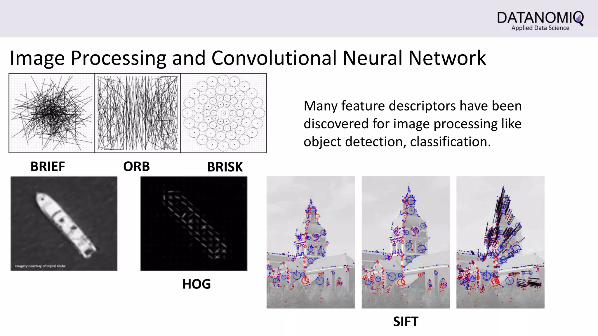
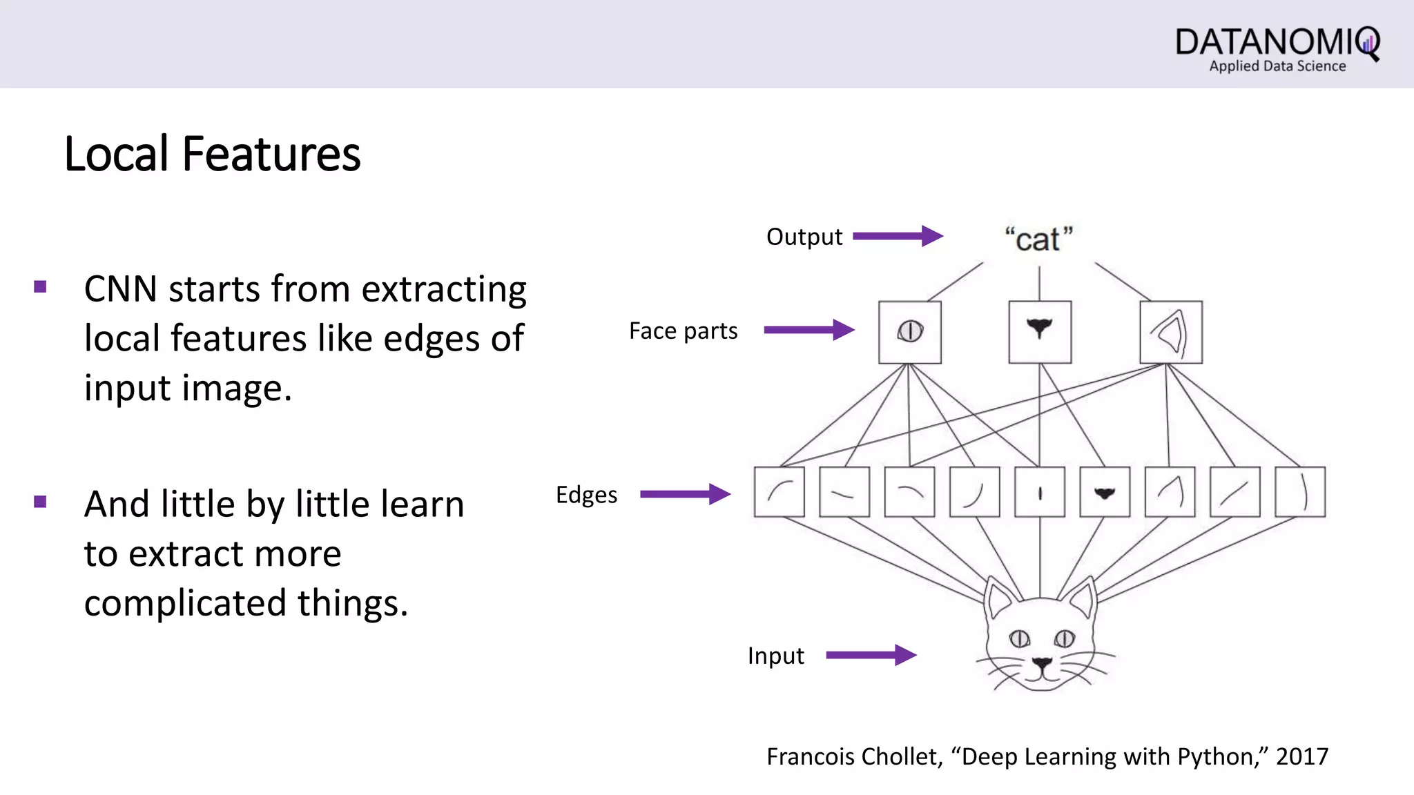
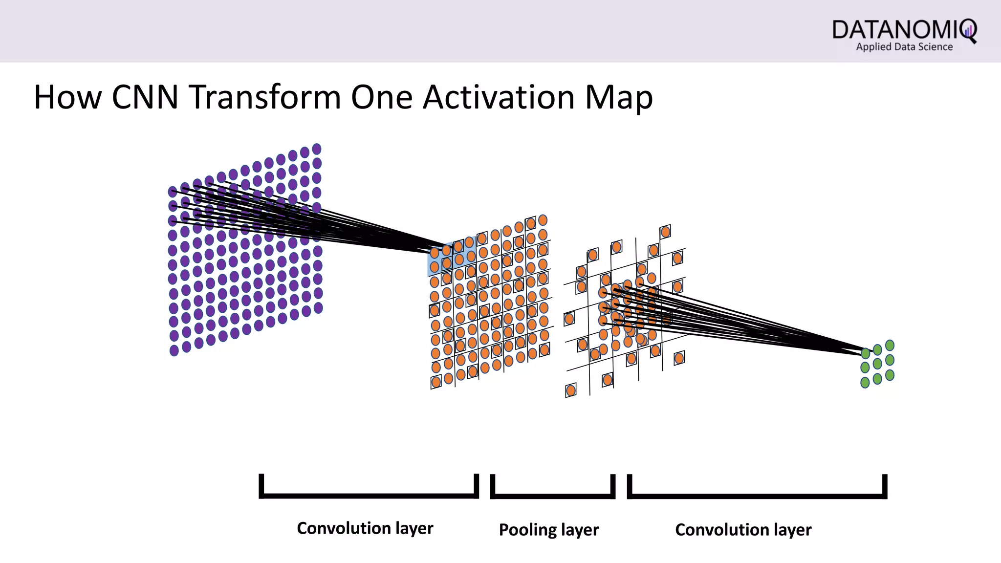
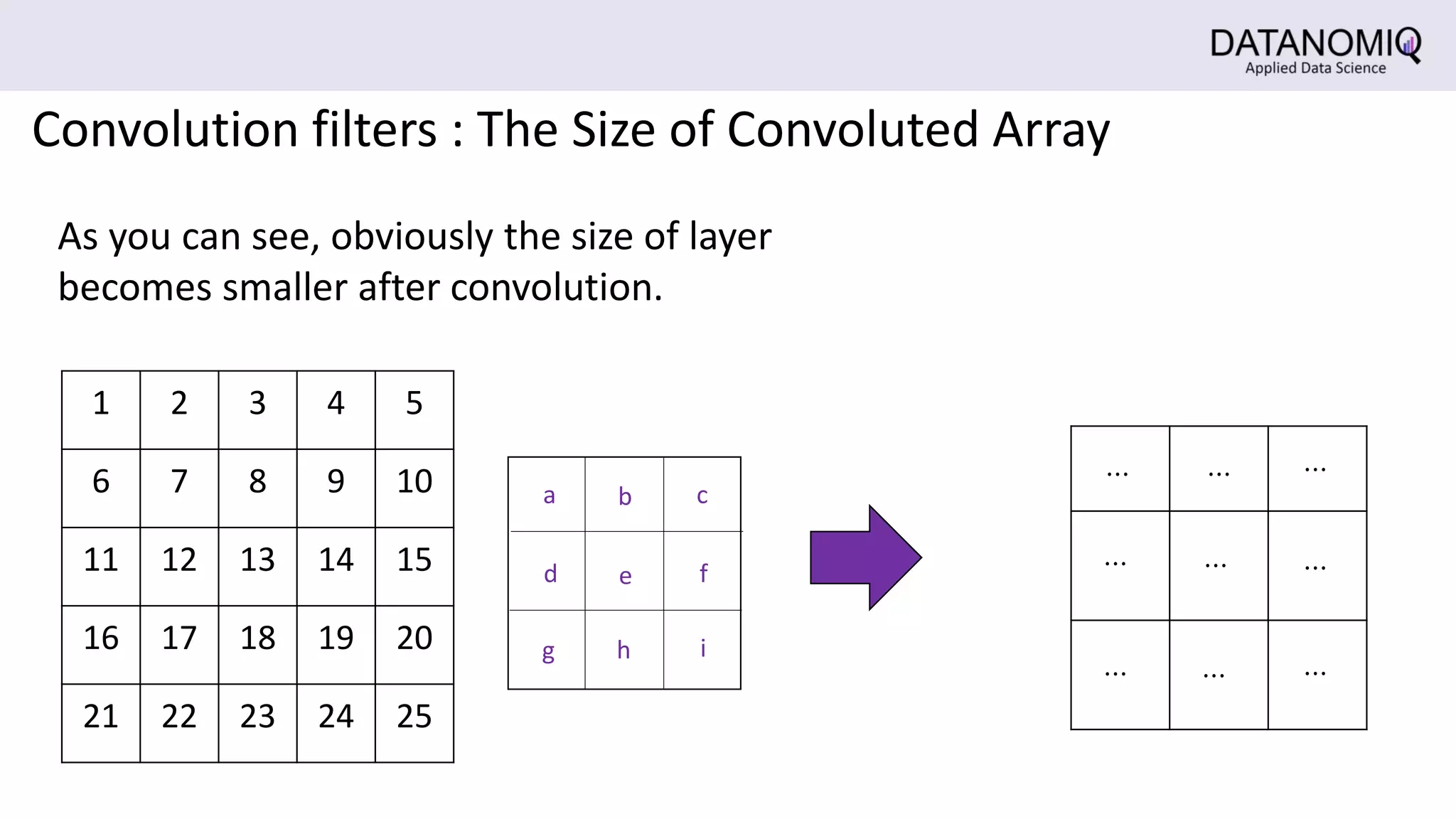
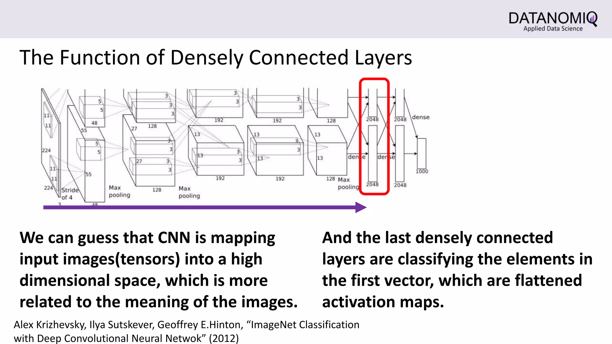
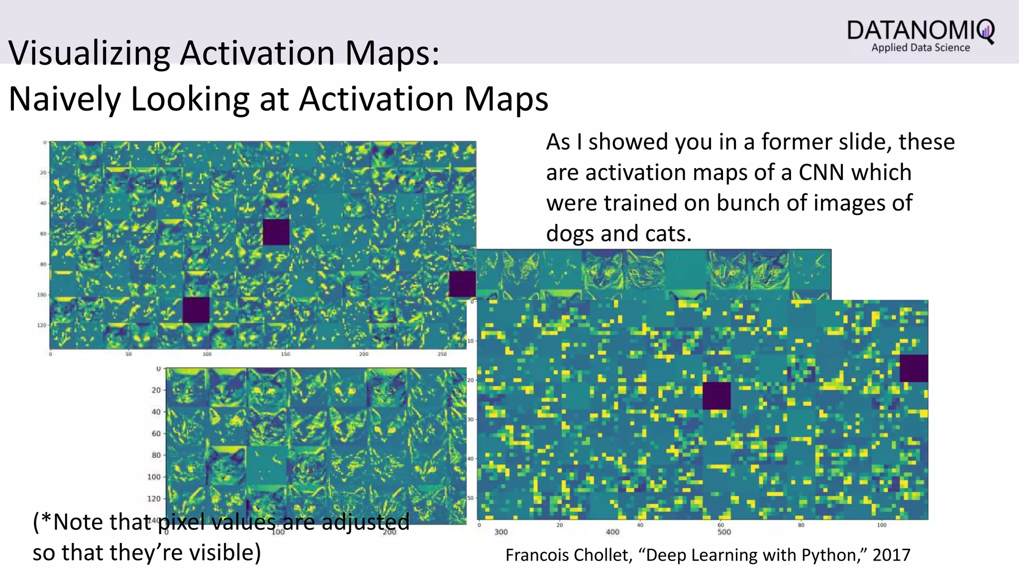
DATANOMIQ GmbH | Franklinstr. 11 | 10587 Berlin
Convolutional Neural Network
Image Processing and Convolutional Neural Network
BRIEF ORB BRISK
HOG
SIFT
Many feature descriptors have been
discovered for image processing like
object detection, classification.
 This is why CNN is also often hyped
as AI.
 On the other hand convolutional
neural network(CNN) learns which
feature to learn.
Image Processing and Convolutional Neural Network
Jonathan Huang, Vivek Rahod, “Google AI Blog, Supercharge
your Computer Vision models with the TensorFlow Object
Detection API”, 2017
https://ai.googleblog.com/2017/06/supercharge-your-
computer-vision-models.html
Image Processing and Convolutional Neural Network
 So please keep it in mind that
convolutional neural network
in just one of the solutions,
when you have bunch of data
prepared.
 And they’re needed for some
fast operations.
 Even with classical descriptors,
you can do a lot of cool stuff.
Classifying MNIST Dataset with
Densely Connected Layers
Black and white images
of 28*28 = 784 pixels
伊藤真、「Pythonで動かして学ぶ!あたらしい機械学習の教科書」、2018
⋮
⋮
⋮
⋮
⋮
⋮
⋮
⋮
Densely Connected Layers
- What is the Input?
0
0
0
0
⋮
⋮
⋮
0.2
0.3
⋮
⋮
⋮
⋮
⋮
⋮
⋮
0
0
Flattening
3%
⋮
⋮
⋮
⋮
83%
⋮
⋮
⋮
⋮
⋮
5%
784-d
vector
16-d
vector
10-d
vector
‘5’
⋮
⋮
⋮
⋮
⋮
⋮
⋮
⋮
⋮
Probability vector by
sigmoid functions
Naive Image Classification with
Densely Connected Layers ERRORS
You can achieve about
90% accuracy with
densely connected layers.
伊藤真、「Pythonで動かして学ぶ!あたらしい機械学習の教科書」、2018
Is this the way we
perceive an image?....
1.0
1.0
1.0
1.0
⋮
⋮
⋮
0.2
0.3
⋮
⋮
⋮
⋮
⋮
⋮
⋮
1.0
1.0
Flattening
Input
Probably,
NO
⋮
⋮
⋮
⋮
⋮
⋮
⋮
⋮
⋮
Neurons in CNN
Pixels of input images are neurons in CNN
Question : What’s the problems of
naively inputting an image as a vector?
 The more separate
pixels are, the less likely
they have correlations.
⋮
⋮
⋮
⋮
⋮
⋮
⋮
⋮
⋮
⋮
⋮
⋮
⋮
 Input vectors can change
drastically even if the inputs
are the pictures of the same
objects.
 Computationally
expensive.
 If you use a 150*150=22500
pixel image.
Why CNN? : computation cost
 If you naively flatten this image, it
is a 22500-d vector, which can be
too much for densely connected
layers.
 In practice, input images are colored,
so it has RGB channels. Then, the
input vector is 22500*3-d vector
Why CNN? : input vectors can be totally different if
the object in the picture shifts
0.4
0.3
0.3
0.7
⋮
⋮
⋮
0.2
0.3
⋮
⋮
⋮
⋮
⋮
⋮
⋮
0.5
0.6
0.5
0.7
0.8
0.9
⋮
⋮
⋮
0.2
0.3
⋮
⋮
⋮
⋮
⋮
⋮
⋮
0.4
1.0
⋮
Why CNN? : The more separate pixels are,
the less likely they have correlations.
 This neuron contains
information from every
input neuron.
 But it is likely that separate
two pixels don’t have so
much correlations.
Local Features
 CNN starts from extracting
local features like edges of
input image.
Input
Edges
Face parts
Output
Francois Chollet, “Deep Learning with Python,” 2017
 And little by little learn
to extract more
complicated things.
Local Features : more concretely
These are activation maps of a CNN
which were trained on bunch of
images of dogs and cats.
Francois Chollet, “Deep Learning with Python,” 2017
*Note that pixel values are adjusted
so that they’re visible
Convolution layer Convolution layerPooling layer
How CNN Transform One Activation Map
Convolution filters
Of course each of lines
have a weight, as well as
densely connected layers.
Convolution filters
Convolution filters
Convolution filters : let’s think
about general 3*3 filter
1 2 3 4 5
6 7 8 9 10
11 12 13 14 15
16 17 18 19 20
21 22 23 24 25
a b c
g
ed f
ih
a + 2*b + 3*c + 6*d + 7*e +
8*f + 11*d + 12*h + 13*i
2*a + 3*b + 4*c + 7*d + 8*e
+ 9*f + 12*d + 13*h + 14*i
13*a + 14*b + 15*c + 18*d +
19*e + 20*f + 23*d + 24*h + 25*i
⋯
⋯
⋯ ⋯ ⋯
⋯
Sobel Operation :
Simple Example of Convolution Filter
1 0 -1
2 0 -2
1 0 -1
1 2 1
0 0 0
-1 -2 -1
Convolution by filters is one
of the simplest operations in
image processing.
Wasabi : one of
three cats in Tamura family.
Detecting
vertical
edges
Detecting
horizontal
edges
Convolution filters : The Size of Convoluted Array
1 2 3 4 5
6 7 8 9 10
11 12 13 14 15
16 17 18 19 20
21 22 23 24 25
a b c
g
ed f
ih
⋯
⋯
⋯ ⋯ ⋯
⋯
⋯⋯
⋯
As you can see, obviously the size of layer
becomes smaller after convolution.
Convolution filters : The Size of Convoluted Array
1 2 3 4 5
6 7 8 9 10
11 12 13 14 15
16 17 18 19 20
21 22 23 24 25
a b c
g
ed f
ih
⋯ ⋯
⋯⋯
If you skip some some blocks, the convoluted
layer also gets smaller. This is called “stride.”
(In the case bellow, stride 2)
a b c
g
ed f
ih
a b c
g
ed f
ih
a b c
g
ed f
ih
Convolution filters : The Size of Convoluted Array
a b c
g
ed f
ih
⋯ ⋯ ⋯⋯
 But if you expand the the original array with blocks of zeros in the
margin, the convoluted array doesn’t shrink(in case of stride 1).
0 0 0 0 0 0
0 1 2 3 4 0
0 5 6 7 8 0
0 9 10 11 12 0
0 13 14 15 16 0
0 0 0 0 0 0
⋯ ⋯ ⋯⋯
⋯ ⋯ ⋯⋯
⋯ ⋯ ⋯⋯
 This is called ”zero padding.”
Convolution arithmetic
 It might be nice to think by
yourself about what convolution
is like when you apply various
size of filters and various types of
stride and padding.
 Honestly, these are boring topics
to show in a lecture.
Recommended
material available
online
Pooling : Let’s Think about 2*2 Batches
1 2 3 4
5 6 7 8
9 10 11 12
13 14 15 16
Max pooling Average pooling
3.5 5.5
11.5 13.5
6 8
14 16
Pooling is just dividing a matrix into batches with the same size,
and calculate the maximum value or average in the batch.
Pooling : 2*2 Max Pooling in Practice
It’s like watching the history
of Nintendo backward.
Pooling  With pooling layer, you can
blur the effects of some
shifts of objects.
*Rather, this looks like Spelunker
 And pooled images are
closer to how people
recognize things. Many
people still would be able to
recognize they’re Mario
even after some poolings.
...I don’t want to draw the actual
network on PowerPoint.
This is an image of
what the entire
network looks like
Please open your
smartphone or laptop
and open a browser.
Cool Visualization of CNN
Please search
”2d visualization
of cnn”
http://scs.ryerson.ca/
~aharley/vis/conv/flat
.html
Convolution Layers in General : More Exactly
⋯
⋯
Input activation
maps
⋮
Output activation
maps
原田達也、「機械学習プロフェッショ
ナルシリーズ 画像認識」、2017
These are activations
calculated by forward
propagation.
You calculate these FILTERS
by back propagation.
⋮
⋮ *Note that the number
of output activation
maps are the same as
filters.
原田達也、「機械学習プロフェッショナルシリーズ 画像認識」、2017
Convolution Layers in General : More Exactly
Forward Propagation of CNN :
More Mathematically
⋯
⋮
原田達也、「機械学習プロフェッショナルシリーズ 画像認識」、2017
 Forward propagation is relatively simple.
 In this slide, a set all the
activation maps in the No. layer
is expressed as
 Basically you use convolution layer or
backprop layer to invert to
Forward Propagation of
CNN : Convolution Layer
原田達也、「機械学習プロフェッショナルシリーズ 画像認識」、2017
⋮
⋮
Forward Propagation of
CNN : Pooling Layer
原田達也、「機械学習プロフェッショナルシリーズ 画像認識」、2017
Back Propagation of CNN
原田達也、「機械学習プロフェッショナルシリーズ 画像認識」、2017
⋮
⋮
⋮
 Back propagation of CNN is basically the
same as that of densely connected layers.
 But you have you be careful because you
have to care about shared weight.
 I don’t have any cool animations or
something for this topic. Please be
patient to follow each equation. It’s also
important for mathematics.
Back Propagation of CNN
原田達也、「機械学習プロフェッショナルシリーズ 画像認識」、2017
⋮
⋮
⋮
First just as well as backprop of densely
connected layers, calculate the partial
differentiation of a loss function with
respect to each weight.
*Pay attention to which a are
functions of w, and apply chain
rule.
Back Propagation of CNN
原田達也、「機械学習プロフェッショナルシリーズ 画像認識」、2017
⋮
⋮
⋮
∵
Let , then
Back Propagation of CNN
原田達也、「機械学習プロフェッショナルシリーズ 画像認識」、2017
⋮
⋮
⋮
∵
Back Propagation of CNN
原田達也、「機械学習プロフェッショナルシリーズ 画像認識」、2017
⋮
⋮
⋮
Hence
Visualizing CNN
Why can CNN recognize images?
In fact people didn’t exactly know why CNN
outperformed former image classification methods.
 It is said that the structure of CNN is based
on that a model of image recognition
system named Neocognitron.
Visualizing CNN : A Very Brief History of CNN
 You can see that the ideas of shared
weights(convolution) and pooling had
already existed at this point.
Kunihiko Fukushima, “Neocognitron: A Self-organizing
Neural Network Model for a Mechanism of Pattern
Recognition Unaffected by Shift in Position ,” 1980
Visualizing CNN : A Very Brief History of CNN
 And Neocognitron imitates brain structure
proposed by Hubel and Wiesel.
 According to them, visual cortex
simple cells and complex cells are
placed alternately in visual cortex.
 They inserted a microelectronode
into the brain of an anesthetized
cat and recorded which type of
images cause responses in brain.
D. H. Hubel, T. N. Wiesel, Receptive Field of Single Neurons
in the Cat’s Striate Cortex, 1959 https://www.youtube.com/watch?v=IOHayh06LJ4
The Function of Densely Connected Layers
Activating
⋮
⋮
⋮
⋮
⋮
⋮
⋯
⋮
⋮
⋮
4096-d
vectorsAlex Krizhevsky, Ilya Sutskever, Geoffrey E.Hinton, “ImageNet
Classification with Deep Convolutional Neural Netwok” (2012)
AlexNet
The Function of Densely Connected Layers
⋮
⋮
⋮
⋮
⋮
⋮
⋮
⋮
⋮
⋮
⋮
⋮
⋮
⋮
⋮
⋮
⋮
⋮
⋮
⋮
⋮
⋮
⋮
⋮
⋮
⋮
⋮
⋮
⋮
⋮
⋮
⋮
⋮
If you apply clustering to those 4096-d vectors,
the pictures with similar objects gather.
But they’re not
necessarily close
in terms of pixels.
*Keep it in mind that
this is 4096-d spaceAlex Krizhevsky, Ilya Sutskever, Geoffrey E.Hinton, “ImageNet
Classification with Deep Convolutional Neural Netwok” (2012)
⋮
⋮
⋮
⋮
⋮
⋮
⋮
⋮
⋮
⋮
⋮
⋮
If you apply this clustering to much more images,
you can get cool maps of images classified by CNN
*The examples above use dimension reduction method called
t-SNE to plot 4096 vectors to 2 dimensional coordinates.
t-SNE visualization of CNN codes
https://cs.stanford.edu/people/karpathy/cnnembed/
The Function of Densely Connected Layers
We can guess that CNN is mapping
input images(tensors) into a high
dimensional space, which is more
related to the meaning of the images.
And the last densely connected
layers are classifying the elements in
the first vector, which are flattened
activation maps.
Alex Krizhevsky, Ilya Sutskever, Geoffrey E.Hinton, “ImageNet Classification
with Deep Convolutional Neural Netwok” (2012)
Visualizing Activation Maps:
Naively Looking at Activation Maps
As I showed you in a former slide, these
are activation maps of a CNN which
were trained on bunch of images of
dogs and cats.
(*Note that pixel values are adjusted
so that they’re visible) Francois Chollet, “Deep Learning with Python,” 2017
Visualizing Activation Maps: Naively Looking at Maps
Francois Chollet, “Deep Learning with Python,” 2017
 This is the activation maps
of the last hidden layer of
a dog-cat classification
after pooling.
 Just looking at activation
maps doesn’t give you so
much insight.
Visualizing Activation Maps : Using Deconvnet
Matthew D. Zeiler, Rob Fergus, “Visualizing and Understanding Convolutional Networks” (2013)
 This is a model of deconvolutional neural
network proposed Zeiler and Fergus
 This is applying pooling and convolution
to an activation map backward(I’m not
going to explain how it does in this
lecture).
 If you turn all other activation maps to
zero and apply deconvnets to a certain
activation map, you can visualize which
part of image caused the activation
most on input pixels.
Visualizing Activation Maps : Using Deconvnet
Matthew D. Zeiler, Rob Fergus, “Visualizing and Understanding Convolutional Networks” (2013)
An activation
map
Top 9 image
patches receptive
to the activation.
Deconvnet
Visualizing Activation Maps : Using Deconvnet
Matthew D. Zeiler, Rob Fergus, “Visualizing and Understanding Convolutional Networks” (2013)
Question : These 9 patches are the most receptive one activation map.
What is the analogy of those 9 patches?
Deconvnet shows that
the grass in the
background caused the
best activation of the
activation map.

Illustrative Introductory CNN

  • 1.
    DATANOMIQ GmbH |Franklinstr. 11 | 10587 Berlin Convolutional Neural Network
  • 2.
    Image Processing andConvolutional Neural Network BRIEF ORB BRISK HOG SIFT Many feature descriptors have been discovered for image processing like object detection, classification.
  • 3.
     This iswhy CNN is also often hyped as AI.  On the other hand convolutional neural network(CNN) learns which feature to learn. Image Processing and Convolutional Neural Network Jonathan Huang, Vivek Rahod, “Google AI Blog, Supercharge your Computer Vision models with the TensorFlow Object Detection API”, 2017 https://ai.googleblog.com/2017/06/supercharge-your- computer-vision-models.html
  • 4.
    Image Processing andConvolutional Neural Network  So please keep it in mind that convolutional neural network in just one of the solutions, when you have bunch of data prepared.  And they’re needed for some fast operations.  Even with classical descriptors, you can do a lot of cool stuff.
  • 5.
    Classifying MNIST Datasetwith Densely Connected Layers Black and white images of 28*28 = 784 pixels 伊藤真、「Pythonで動かして学ぶ!あたらしい機械学習の教科書」、2018 ⋮ ⋮ ⋮ ⋮
  • 6.
    ⋮ ⋮ ⋮ ⋮ Densely Connected Layers -What is the Input? 0 0 0 0 ⋮ ⋮ ⋮ 0.2 0.3 ⋮ ⋮ ⋮ ⋮ ⋮ ⋮ ⋮ 0 0 Flattening 3% ⋮ ⋮ ⋮ ⋮ 83% ⋮ ⋮ ⋮ ⋮ ⋮ 5% 784-d vector 16-d vector 10-d vector ‘5’ ⋮ ⋮ ⋮ ⋮ ⋮ ⋮ ⋮ ⋮ ⋮ Probability vector by sigmoid functions
  • 7.
    Naive Image Classificationwith Densely Connected Layers ERRORS You can achieve about 90% accuracy with densely connected layers. 伊藤真、「Pythonで動かして学ぶ!あたらしい機械学習の教科書」、2018
  • 8.
    Is this theway we perceive an image?.... 1.0 1.0 1.0 1.0 ⋮ ⋮ ⋮ 0.2 0.3 ⋮ ⋮ ⋮ ⋮ ⋮ ⋮ ⋮ 1.0 1.0 Flattening Input Probably, NO ⋮ ⋮ ⋮ ⋮ ⋮ ⋮ ⋮ ⋮ ⋮
  • 9.
    Neurons in CNN Pixelsof input images are neurons in CNN
  • 10.
    Question : What’sthe problems of naively inputting an image as a vector?  The more separate pixels are, the less likely they have correlations. ⋮ ⋮ ⋮ ⋮ ⋮ ⋮ ⋮ ⋮ ⋮ ⋮ ⋮ ⋮ ⋮  Input vectors can change drastically even if the inputs are the pictures of the same objects.  Computationally expensive.
  • 11.
     If youuse a 150*150=22500 pixel image. Why CNN? : computation cost  If you naively flatten this image, it is a 22500-d vector, which can be too much for densely connected layers.  In practice, input images are colored, so it has RGB channels. Then, the input vector is 22500*3-d vector
  • 12.
    Why CNN? :input vectors can be totally different if the object in the picture shifts 0.4 0.3 0.3 0.7 ⋮ ⋮ ⋮ 0.2 0.3 ⋮ ⋮ ⋮ ⋮ ⋮ ⋮ ⋮ 0.5 0.6 0.5 0.7 0.8 0.9 ⋮ ⋮ ⋮ 0.2 0.3 ⋮ ⋮ ⋮ ⋮ ⋮ ⋮ ⋮ 0.4 1.0
  • 13.
    ⋮ Why CNN? :The more separate pixels are, the less likely they have correlations.  This neuron contains information from every input neuron.  But it is likely that separate two pixels don’t have so much correlations.
  • 14.
    Local Features  CNNstarts from extracting local features like edges of input image. Input Edges Face parts Output Francois Chollet, “Deep Learning with Python,” 2017  And little by little learn to extract more complicated things.
  • 15.
    Local Features :more concretely These are activation maps of a CNN which were trained on bunch of images of dogs and cats. Francois Chollet, “Deep Learning with Python,” 2017 *Note that pixel values are adjusted so that they’re visible
  • 16.
    Convolution layer ConvolutionlayerPooling layer How CNN Transform One Activation Map
  • 17.
    Convolution filters Of courseeach of lines have a weight, as well as densely connected layers.
  • 18.
  • 19.
  • 20.
    Convolution filters :let’s think about general 3*3 filter 1 2 3 4 5 6 7 8 9 10 11 12 13 14 15 16 17 18 19 20 21 22 23 24 25 a b c g ed f ih a + 2*b + 3*c + 6*d + 7*e + 8*f + 11*d + 12*h + 13*i 2*a + 3*b + 4*c + 7*d + 8*e + 9*f + 12*d + 13*h + 14*i 13*a + 14*b + 15*c + 18*d + 19*e + 20*f + 23*d + 24*h + 25*i ⋯ ⋯ ⋯ ⋯ ⋯ ⋯
  • 21.
    Sobel Operation : SimpleExample of Convolution Filter 1 0 -1 2 0 -2 1 0 -1 1 2 1 0 0 0 -1 -2 -1 Convolution by filters is one of the simplest operations in image processing. Wasabi : one of three cats in Tamura family. Detecting vertical edges Detecting horizontal edges
  • 22.
    Convolution filters :The Size of Convoluted Array 1 2 3 4 5 6 7 8 9 10 11 12 13 14 15 16 17 18 19 20 21 22 23 24 25 a b c g ed f ih ⋯ ⋯ ⋯ ⋯ ⋯ ⋯ ⋯⋯ ⋯ As you can see, obviously the size of layer becomes smaller after convolution.
  • 23.
    Convolution filters :The Size of Convoluted Array 1 2 3 4 5 6 7 8 9 10 11 12 13 14 15 16 17 18 19 20 21 22 23 24 25 a b c g ed f ih ⋯ ⋯ ⋯⋯ If you skip some some blocks, the convoluted layer also gets smaller. This is called “stride.” (In the case bellow, stride 2) a b c g ed f ih a b c g ed f ih a b c g ed f ih
  • 24.
    Convolution filters :The Size of Convoluted Array a b c g ed f ih ⋯ ⋯ ⋯⋯  But if you expand the the original array with blocks of zeros in the margin, the convoluted array doesn’t shrink(in case of stride 1). 0 0 0 0 0 0 0 1 2 3 4 0 0 5 6 7 8 0 0 9 10 11 12 0 0 13 14 15 16 0 0 0 0 0 0 0 ⋯ ⋯ ⋯⋯ ⋯ ⋯ ⋯⋯ ⋯ ⋯ ⋯⋯  This is called ”zero padding.”
  • 25.
    Convolution arithmetic  Itmight be nice to think by yourself about what convolution is like when you apply various size of filters and various types of stride and padding.  Honestly, these are boring topics to show in a lecture. Recommended material available online
  • 26.
    Pooling : Let’sThink about 2*2 Batches 1 2 3 4 5 6 7 8 9 10 11 12 13 14 15 16 Max pooling Average pooling 3.5 5.5 11.5 13.5 6 8 14 16 Pooling is just dividing a matrix into batches with the same size, and calculate the maximum value or average in the batch.
  • 27.
    Pooling : 2*2Max Pooling in Practice It’s like watching the history of Nintendo backward.
  • 28.
    Pooling  Withpooling layer, you can blur the effects of some shifts of objects. *Rather, this looks like Spelunker  And pooled images are closer to how people recognize things. Many people still would be able to recognize they’re Mario even after some poolings.
  • 29.
    ...I don’t wantto draw the actual network on PowerPoint. This is an image of what the entire network looks like
  • 30.
    Please open your smartphoneor laptop and open a browser.
  • 31.
    Cool Visualization ofCNN Please search ”2d visualization of cnn” http://scs.ryerson.ca/ ~aharley/vis/conv/flat .html
  • 32.
    Convolution Layers inGeneral : More Exactly ⋯ ⋯ Input activation maps ⋮ Output activation maps 原田達也、「機械学習プロフェッショ ナルシリーズ 画像認識」、2017
  • 33.
    These are activations calculatedby forward propagation. You calculate these FILTERS by back propagation. ⋮ ⋮ *Note that the number of output activation maps are the same as filters. 原田達也、「機械学習プロフェッショナルシリーズ 画像認識」、2017 Convolution Layers in General : More Exactly
  • 34.
    Forward Propagation ofCNN : More Mathematically ⋯ ⋮ 原田達也、「機械学習プロフェッショナルシリーズ 画像認識」、2017  Forward propagation is relatively simple.  In this slide, a set all the activation maps in the No. layer is expressed as  Basically you use convolution layer or backprop layer to invert to
  • 35.
    Forward Propagation of CNN: Convolution Layer 原田達也、「機械学習プロフェッショナルシリーズ 画像認識」、2017 ⋮ ⋮
  • 36.
    Forward Propagation of CNN: Pooling Layer 原田達也、「機械学習プロフェッショナルシリーズ 画像認識」、2017
  • 37.
    Back Propagation ofCNN 原田達也、「機械学習プロフェッショナルシリーズ 画像認識」、2017 ⋮ ⋮ ⋮  Back propagation of CNN is basically the same as that of densely connected layers.  But you have you be careful because you have to care about shared weight.  I don’t have any cool animations or something for this topic. Please be patient to follow each equation. It’s also important for mathematics.
  • 38.
    Back Propagation ofCNN 原田達也、「機械学習プロフェッショナルシリーズ 画像認識」、2017 ⋮ ⋮ ⋮ First just as well as backprop of densely connected layers, calculate the partial differentiation of a loss function with respect to each weight. *Pay attention to which a are functions of w, and apply chain rule.
  • 39.
    Back Propagation ofCNN 原田達也、「機械学習プロフェッショナルシリーズ 画像認識」、2017 ⋮ ⋮ ⋮ ∵ Let , then
  • 40.
    Back Propagation ofCNN 原田達也、「機械学習プロフェッショナルシリーズ 画像認識」、2017 ⋮ ⋮ ⋮ ∵
  • 41.
    Back Propagation ofCNN 原田達也、「機械学習プロフェッショナルシリーズ 画像認識」、2017 ⋮ ⋮ ⋮ Hence
  • 42.
    Visualizing CNN Why canCNN recognize images? In fact people didn’t exactly know why CNN outperformed former image classification methods.
  • 43.
     It issaid that the structure of CNN is based on that a model of image recognition system named Neocognitron. Visualizing CNN : A Very Brief History of CNN  You can see that the ideas of shared weights(convolution) and pooling had already existed at this point. Kunihiko Fukushima, “Neocognitron: A Self-organizing Neural Network Model for a Mechanism of Pattern Recognition Unaffected by Shift in Position ,” 1980
  • 44.
    Visualizing CNN :A Very Brief History of CNN  And Neocognitron imitates brain structure proposed by Hubel and Wiesel.  According to them, visual cortex simple cells and complex cells are placed alternately in visual cortex.  They inserted a microelectronode into the brain of an anesthetized cat and recorded which type of images cause responses in brain. D. H. Hubel, T. N. Wiesel, Receptive Field of Single Neurons in the Cat’s Striate Cortex, 1959 https://www.youtube.com/watch?v=IOHayh06LJ4
  • 45.
    The Function ofDensely Connected Layers Activating ⋮ ⋮ ⋮ ⋮ ⋮ ⋮ ⋯ ⋮ ⋮ ⋮ 4096-d vectorsAlex Krizhevsky, Ilya Sutskever, Geoffrey E.Hinton, “ImageNet Classification with Deep Convolutional Neural Netwok” (2012) AlexNet
  • 46.
    The Function ofDensely Connected Layers ⋮ ⋮ ⋮ ⋮ ⋮ ⋮ ⋮ ⋮ ⋮ ⋮ ⋮ ⋮ ⋮ ⋮ ⋮ ⋮ ⋮ ⋮ ⋮ ⋮ ⋮ ⋮ ⋮ ⋮ ⋮ ⋮ ⋮ ⋮ ⋮ ⋮ ⋮ ⋮ ⋮ If you apply clustering to those 4096-d vectors, the pictures with similar objects gather. But they’re not necessarily close in terms of pixels. *Keep it in mind that this is 4096-d spaceAlex Krizhevsky, Ilya Sutskever, Geoffrey E.Hinton, “ImageNet Classification with Deep Convolutional Neural Netwok” (2012) ⋮ ⋮ ⋮ ⋮ ⋮ ⋮ ⋮ ⋮ ⋮ ⋮ ⋮ ⋮
  • 47.
    If you applythis clustering to much more images, you can get cool maps of images classified by CNN *The examples above use dimension reduction method called t-SNE to plot 4096 vectors to 2 dimensional coordinates. t-SNE visualization of CNN codes https://cs.stanford.edu/people/karpathy/cnnembed/
  • 48.
    The Function ofDensely Connected Layers We can guess that CNN is mapping input images(tensors) into a high dimensional space, which is more related to the meaning of the images. And the last densely connected layers are classifying the elements in the first vector, which are flattened activation maps. Alex Krizhevsky, Ilya Sutskever, Geoffrey E.Hinton, “ImageNet Classification with Deep Convolutional Neural Netwok” (2012)
  • 49.
    Visualizing Activation Maps: NaivelyLooking at Activation Maps As I showed you in a former slide, these are activation maps of a CNN which were trained on bunch of images of dogs and cats. (*Note that pixel values are adjusted so that they’re visible) Francois Chollet, “Deep Learning with Python,” 2017
  • 50.
    Visualizing Activation Maps:Naively Looking at Maps Francois Chollet, “Deep Learning with Python,” 2017  This is the activation maps of the last hidden layer of a dog-cat classification after pooling.  Just looking at activation maps doesn’t give you so much insight.
  • 51.
    Visualizing Activation Maps: Using Deconvnet Matthew D. Zeiler, Rob Fergus, “Visualizing and Understanding Convolutional Networks” (2013)  This is a model of deconvolutional neural network proposed Zeiler and Fergus  This is applying pooling and convolution to an activation map backward(I’m not going to explain how it does in this lecture).  If you turn all other activation maps to zero and apply deconvnets to a certain activation map, you can visualize which part of image caused the activation most on input pixels.
  • 52.
    Visualizing Activation Maps: Using Deconvnet Matthew D. Zeiler, Rob Fergus, “Visualizing and Understanding Convolutional Networks” (2013) An activation map Top 9 image patches receptive to the activation. Deconvnet
  • 53.
    Visualizing Activation Maps: Using Deconvnet Matthew D. Zeiler, Rob Fergus, “Visualizing and Understanding Convolutional Networks” (2013) Question : These 9 patches are the most receptive one activation map. What is the analogy of those 9 patches? Deconvnet shows that the grass in the background caused the best activation of the activation map.