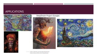
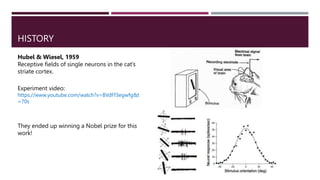
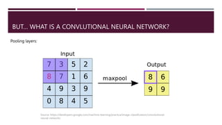
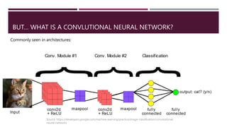
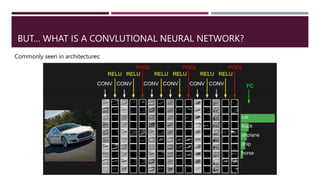
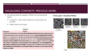
This document provides an overview of convolutional neural networks (CNNs or ConvNets). It discusses the history of ConvNets from their origins in modeling the visual cortex to modern applications in computer vision tasks. The document explains what ConvNets are through their use of filters, activation maps, and pooling layers. It also discusses methods for visualizing and understanding what different layers of ConvNets are learning from images.

1. MACHINES THAT SEE
Visualizing and Understanding Convolutional Neural Networks
Mohamed Ali
Habib

2. CONTENTS
 Motivation: Why do ConvNets exist?
 History.
 What is a ConvNet?
 Intuition: What are ConvNets learning?
 Visualizing layers.
 Applications.
 References.

3. WHY DO THEY EXIST?
Common computer vision tasks:
Source: https://medium.com/zylapp/review-of-deep-learning-algorithms-for-object-detection-
c1f3d437b852

4. HISTORY
Hubel & Wiesel, 1959
Receptive fields of single neurons in the cat’s
striate cortex.
They ended up winning a Nobel prize for this
work!
Experiment video:
https://www.youtube.com/watch?v=8VdFf3egwfg&t
=70s

5. HISTORY
1998.. First ConvNet paper!
Gradient-based learning applied to document recognition [LeCun, Bottou, Bengio, Haffner1998]
https://ieeexplore.ieee.org/document/726791
LeNet-5
• Small architecture.
• 60K parameters.
• Used backpropagation.
6 5x5 filters
s=1
Average
pooling
16 5x5 filters
s=1
Average
pooling FC: 120
neurons
FC: 84
neurons
𝑦: 10 outputs (digits)

6. HISTORY
2012.. AlexNet: One of the most impactful papers in computer vision!
ImageNet Classification with Deep Convolutional Neural Networks [Krizhevsky, Sutskever, Hinton, 2012]
https://papers.nips.cc/paper/2012/hash/c399862d3b9d6b76c8436e924a68c45b-Abstract.html
• Winner of ImageNet Competition in 2012.
• Compared to LeNet-5:
• Activation function: ReLU
• Deeper ~60M parameters
• More Data.
• GPU Computation.
• Regularization strategies: Dropout.
AlexNet
It was all about scale.
https://www.image-
net.org/

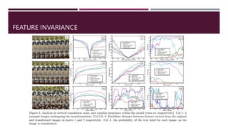
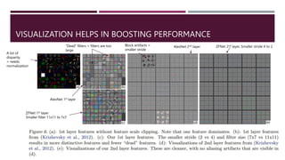
7. HISTORY
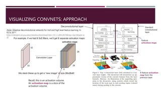
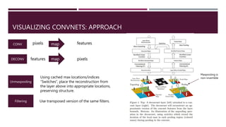
2013.. ZFNet
Visualizing and Understanding Convolutional Networks [Zeiler, Fergus, NYU, 2013]
https://arxiv.org/abs/1311.2901
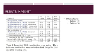
• Winner of ImageNet Competition in 2013.
• Compared to AlexNet:
• Used visualization insights to boost
performance.
• Normalization across feature maps.
• Smaller filter size and stride.
• Initial seed for a startup: resulted in to 2 better
submissions on ImageNet.
ZFNet https://www.image-
net.org/

8. HISTORY
ConvNets surpassed human performance on ImageNet!
• Human error ~ 5%
• SOTA ConvNets ~2-3%
The evolution of the winning entries on the ImageNet Large Scale Visual Recognition Challenge from 2010 to 2015.
Since 2012, CNNs have outperformed hand-crafted descriptors and shallow networks by a large margin.
Source: https://www.researchgate.net/figure/The-evolution-of-the-winning-entries-on-the-ImageNet-Large-Scale-
Visual-Recognition_fig1_321896881
Do you notice the
pattern?

9. BUT… WHAT IS A CONVLUTIONAL NEURAL NETWORK?
Idea: Filter/Kernel sliding over an image (or any volume) computing dot products.
https://analyticsindiamag.com/convolutional-neural-network-image-classification-
overview/
Activation map
Filter
Input image
Applying
many
filters
That’s it! A full convolutional layer.
A representation of the
image.

10. BUT… WHAT IS A CONVLUTIONAL NEURAL NETWORK?
𝑅𝑒𝐿𝑈 𝑥 = max(0, 𝑥)

11. BUT… WHAT IS A CONVLUTIONAL NEURAL NETWORK?
Pooling layers:
Source: https://developers.google.com/machine-learning/practica/image-classification/convolutional-
neural-networks

12. BUT… WHAT IS A CONVLUTIONAL NEURAL NETWORK?
Commonly seen in architectures:
Source: https://developers.google.com/machine-learning/practica/image-classification/convolutional-
neural-networks

13. BUT… WHAT IS A CONVLUTIONAL NEURAL NETWORK?
Commonly seen in architectures:

14. WHAT ARE CNNS LEARNING?
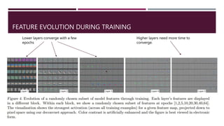
From Yann LeCun slides. Feature visualization of convolutional net trained on ImageNet from [Zeiler & Fergus 2013]:

15. VISUALIZING CONVNETS: PREVIOUS WORK
 Visualizing learned weights of filters of convolutional
layers:
 Limited to 1st layer where projections to pixel space are
possible.
 Higher layers are complex.
Higher
layers
T-SNE:

16. VISUALIZING CONVNETS: WHY?
 Visualizing pros:
 Makes ConvNets more interpretable: proving meaningful representations.
 Helps in boosting performance of current models.

17. VISUALIZING CONVNETS: APPROACH
Recall: this is an activation volume.
An activation map is a slice of the
activation volume.
Feature
activation maps
Standard
convolutional
layer.
Deconvolutional layer
Zeiler, Adaptive deconvolutional networks for mid and high level feature learning. In
ICCV, 2011.
http://citeseerx.ist.psu.edu/viewdoc/download?doi=10.1.1.849.3679&rep=rep1&type=p
df
A feature activation
map from the
previous layer

18. VISUALIZING CONVNETS: APPROACH
CONV pixels map features
DECONV pixels
map
features
Unmaxpooling
Using cached max locations/indices
“Switches”, place the reconstruction from
the layer above into appropriate locations,
preserving structure.
Filtering Use transposed version of the same filters.
Maxpooling is
non-invertible

19. VISUALIZING LAYERS
Feature visualization of convolutional net trained on ImageNet from [Zeiler & Fergus 2013]:

20. VISUALIZING LAYERS
Feature visualization of convolutional net trained on ImageNet from [Zeiler & Fergus 2013]:

21. VISUALIZING LAYERS
Feature visualization of convolutional net trained on ImageNet from [Zeiler & Fergus 2013]:

22. VISUALIZING LAYERS
Feature visualization of convolutional net trained on ImageNet from [Zeiler & Fergus 2013]:

23. VISUALIZING LAYERS
Feature visualization of convolutional net trained on ImageNet from [Zeiler & Fergus 2013]:

24. FEATURE EVOLUTION DURING TRAINING
Lower layers converge with a few
epochs
Higher layers need more time to
converge.

25. FEATURE INVARIANCE

26. VISUALIZATION HELPS IN BOOSTING PERFORMANCE
AlexNet 1st layer
ZFNet 1st layer
Smaller filter 11x11 to 7x7
AlexNet 2nd layer ZFNet 2nd layer, Smaller stride 4 to 2
A lot of
disparity
= needs
normalization
“Dead” filters = filters are too
large
Block artifacts =
smaller stride

27. OCCLUSION SENSITIVITY

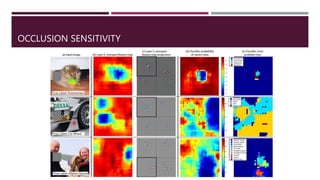
28. OCCLUSION SENSITIVITY
Feature visualization of convolutional net trained on ImageNet from [Zeiler & Fergus
2013]

29. CORRESPONDENCE ANALYSIS
For image 𝑖: ∈𝑖
𝑙
= 𝑥𝑖
𝑙
− 𝑥𝑖
𝑙
∆𝑙=
𝑖,𝑗=1,𝑖≠𝑗
5
ℋ 𝑠𝑖𝑔𝑛 ∈𝑖
𝑙
, 𝑠𝑖𝑔𝑛 ∈𝑗
𝑙
, ℋ: ℎ𝑎𝑚𝑚𝑖𝑛𝑔 𝑑𝑖𝑠𝑡𝑎𝑛𝑐𝑒
• 𝑥𝑖
𝑙
: feature vector for original image at layer 𝑙.
• 𝑥𝑖
𝑙
: feature vector for occluded image at layer 𝑙.

30. ZFNET: TRAINING SETUP
 Built on top of ImageNet [Krizhevsky, Sutskever, Hinton, 2012]
 Labeled dataset: ImageNet (1.3m images & 1000 classes)
 Preprocessing:
 Resize to: 256 × 256
 Subtract per-pixel mean.
 Augmentation: 10 sub-crops.
 Cross-entropy loss function suitable for image classification.
 Parameters:
 Convolutional layers’ filters.
 Weights matrices in fully connected (FC) layers.
 Biases.
 Backpropagation + Stochastic Gradient Descent (SGD)
 Learning rate (starting) 10−2
& momentum of 0.9
 Dropout: rate of 0.5 in FC layers.
 Weights initialized to 10−2
& biases to 0.
 Stopped training after 70 epochs (12 days) on GTX580 GPU.

31. RESULTS: IMAGENET
• Other datasets:
• Caltech-101
• Caltech-256

32. APPLICATIONS
https://selfdrivingcars.mit.edu/
https://github.com/lexfridman/mit-deep-
learning/blob/master/tutorial_driving_scene_segmentation/tutorial_driving_scene_segmentation.ipynb
Driving Scene
Segmentation

33. APPLICATIONS
DeepFace: Closing the Gap to Human-Level Performance in Face Verification:
https://www.cs.toronto.edu/~ranzato/publications/taigman_cvpr14.pdf

34. APPLICATIONS
A Neural Algorithm of Artistic Style:
https://arxiv.org/abs/1508.06576
Source:
https://www.tensorflow.org/tutorials/generative/style_transfer

35. APPLICATIONS
Source: https://github.com/google/deepdream,
https://www.reddit.com/r/deepdream
DeepDream Project (Google)

36. Fun time!
ConvNetJS on CIFAR-10 demo:
https://cs.stanford.edu/people/karpathy/convnetjs/demo/cifar10.html

37. REFERENCES
 Visualizing and Understanding Convolutional Networks:
https://arxiv.org/abs/1311.2901
 Stanford: CS231n Convolutional Neural Networks for Visual
Recognition:
http://cs231n.stanford.edu/
 Honorable mentions:
Understanding Neural Networks Through Deep Visualization
https://arxiv.org/abs/1506.06579
https://github.com/yosinski/deep-visualization-toolbox
Deep Visualization Toolbox
https://youtu.be/AgkfIQ4IGaM
Slides:

38. THANK YOU!