In this presentation…
Introduction to Statistical Learning
Hypothesis Testing in Statistical Learning
Statistical Learning Procedures
Case Study 1: Coffee Sale (t-Test)
Case Study 2: Machine Testing (z-test)
Case Study 3: Perceptual Psychology (-test)
Discussion on Statistical Learning 2
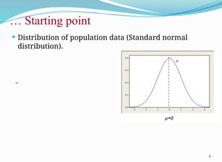
Introduction
5
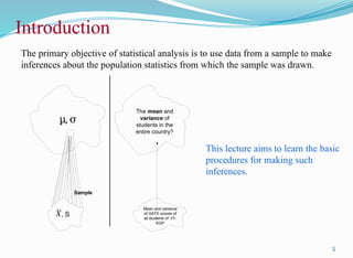
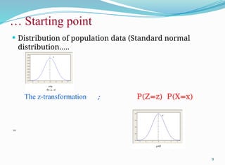
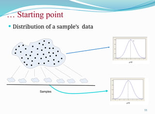
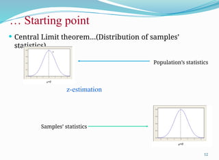
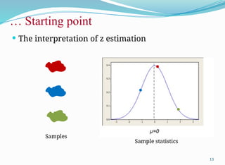
The primary objectiveof statistical analysis is to use data from a sample to make
inferences about the population statistics from which the sample was drawn.
This lecture aims to learn the basic
procedures for making such
inferences.
µ,σ
, S
Sample
Mean and variance
of GATE scores of
all students of IIT-
KGP
The mean and
variance of
students in the
entire country?
𝑋
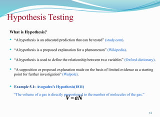
What is Hypothesis?
“A hypothesis is an educated prediction that can be tested” (study.com).
“A hypothesis is a proposed explanation for a phenomenon” (Wikipedia).
“A hypothesis is used to define the relationship between two variables” (Oxford dictionary).
“A supposition or proposed explanation made on the basis of limited evidence as a starting
point for further investigation” (Walpole).
Example 5.1: Avogadro’s Hypothesis(1811)
“The volume of a gas is directly proportional to the number of molecules of the gas.”
15
Hypothesis Testing
𝑽=𝒂𝑵
16.
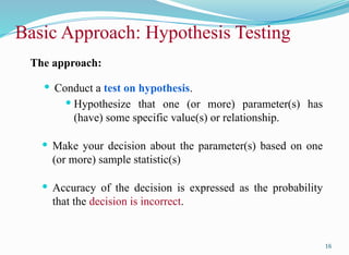
The approach:
Conducta test on hypothesis.
Hypothesize that one (or more) parameter(s) has
(have) some specific value(s) or relationship.
Make your decision about the parameter(s) based on one
(or more) sample statistic(s)
Accuracy of the decision is expressed as the probability
that the decision is incorrect.
16
Basic Approach: Hypothesis Testing
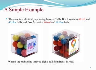
There aretwo identically appearing boxes of balls. Box 1 contains 60 red and
40 blue balls, and Box 2 contains 40 red and 60 blue balls.
18
A Simple Example
What is the probability that you pick a ball from Box 1 is read?
19.
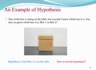
One ofthe box is sitting on the table, but you don’t know which one it is. You
have to guess which box it is: Box 1 or Box 2?
19
An Example of Hypothesis
Hypothesis is that Box 2 is on the table. How to test the hypothesis?
20.
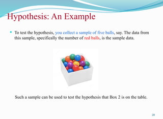
To testthe hypothesis, you collect a sample of five balls, say. The data from
this sample, specifically the number of red balls, is the sample data.
20
Hypothesis: An Example
Such a sample can be used to test the hypothesis that Box 2 is on the table.
21.
Hypothesis isthat
Box 2 is on the table.
H0: p = 0.4
21
Hypothesis: An Example
Such a hypothesis is called Null Hypothesis.
Box 2 contains 40 red and 60 blue balls.
22.
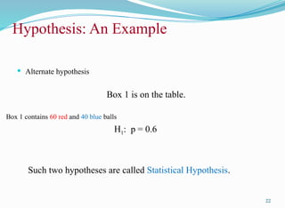
Alternate hypothesis
Box1 is on the table.
H1: p = 0.6
22
Hypothesis: An Example
Such two hypotheses are called Statistical Hypothesis.
Box 1 contains 60 red and 40 blue balls
23.
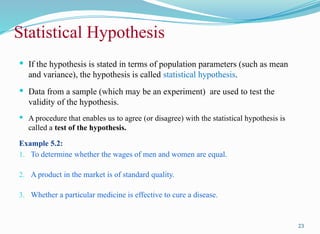
If thehypothesis is stated in terms of population parameters (such as mean
and variance), the hypothesis is called statistical hypothesis.
Data from a sample (which may be an experiment) are used to test the
validity of the hypothesis.
A procedure that enables us to agree (or disagree) with the statistical hypothesis is
called a test of the hypothesis.
Example 5.2:
1. To determine whether the wages of men and women are equal.
2. A product in the market is of standard quality.
3. Whether a particular medicine is effective to cure a disease.
23
Statistical Hypothesis
24.
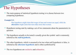
The mainpurpose of statistical hypothesis testing is to choose between two
competing hypotheses.
Example 5.3:
One hypothesis might claim that wages of men and women are equal, while the
alternative might claim that men make more than women.
Hypothesis testing start by making a set of two statements about the parameter(s) in
question.
The hypothesis actually to be tested is usually given the symbol and is commonly
referred as the null hypothesis.
The other hypothesis, which is assumed to be true when null hypothesis is false, is
referred as the alternate hypothesis and is often symbolized by
The two hypotheses are exclusive and exhaustive.
24
The Hypotheses
25.
Example 5.4:
Ministry ofHuman Resource Development (MHRD), Government of India
takes an initiative to improve the country’s human resources and hence set up
23 IIT’s in the country.
To measure the engineering aptitudes of graduates, MHRD conducts GATE
examination for a mark of 1000 in every year. A sample of 300 students who
gave GATE examination in 2021 were collected and the mean is observed as
220.
In this context, statistical hypothesis testing is to determine the mean mark of
the all GATE-2021 examinee.
The two hypotheses in this context are:
25
The Hypotheses
26.
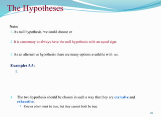
Note:
1. As nullhypothesis, we could choose or
2. It is customary to always have the null hypothesis with an equal sign.
3. As an alternative hypothesis there are many options available with us.
Examples 5.5:
I.
4. The two hypothesis should be chosen in such a way that they are exclusive and
exhaustive.
One or other must be true, but they cannot both be true.
26
The Hypotheses
27.
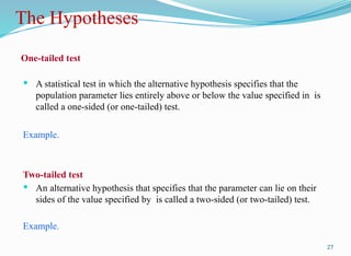
One-tailed test
Astatistical test in which the alternative hypothesis specifies that the
population parameter lies entirely above or below the value specified in is
called a one-sided (or one-tailed) test.
Example.
Two-tailed test
An alternative hypothesis that specifies that the parameter can lie on their
sides of the value specified by is called a two-sided (or two-tailed) test.
Example.
27
The Hypotheses
28.
Note:
In fact, a1-tailed test such as:
is same as
In essence, it does not imply that , etc.
28
The Hypotheses
What about two-tailed test?
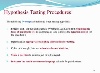
The following fivesteps are followed when testing hypothesis
1. Specify and , the null and alternate hypothesis. Also, decide the significance
level of hypothesis test (it is denoted as and signifies the rejection region for
the specified ).
2. Determine an appropriate sampling distribution for testing.
3. Collect the sample data and calculate the test statistics.
4. Make a decision to either reject or fail to reject .
5. Interpret the result in common language suitable for practitioners.
31
Hypothesis Testing Procedures
32.
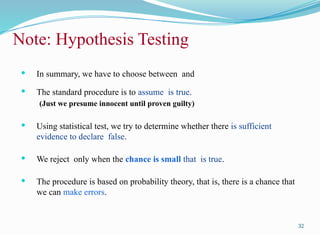
In summary,we have to choose between and
The standard procedure is to assume is true.
(Just we presume innocent until proven guilty)
Using statistical test, we try to determine whether there is sufficient
evidence to declare false.
We reject only when the chance is small that is true.
The procedure is based on probability theory, that is, there is a chance that
we can make errors.
32
Note: Hypothesis Testing
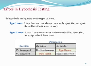
In hypothesis testing,there are two types of errors.
Type I error: A type I error occurs when we incorrectly reject (i.e., we reject
the null hypothesis, when is true).
Type II error: A type II error occurs when we incorrectly fail to reject (i.e.,
we accept when it is not true).
34
Errors in Hypothesis Testing
35.
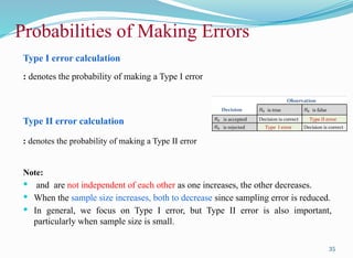
Type I errorcalculation
: denotes the probability of making a Type I error
Type II error calculation
: denotes the probability of making a Type II error
Note:
and are not independent of each other as one increases, the other decreases.
When the sample size increases, both to decrease since sampling error is reduced.
In general, we focus on Type I error, but Type II error is also important,
particularly when sample size is small.
35
Probabilities of Making Errors
36.
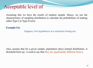
Assuming that wehave the results of random sample. Hence, we use the
characteristics of sampling distribution to calculate the probabilities of making
either Type I or Type II error.
Example 5.6:
Suppose, two hypotheses in a statistical testing are:
Also, assume that for a given sample, population obeys normal distribution. A
threshold limit say is used to say that they are significantly different from a.
36
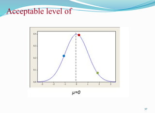
Acceptable level of
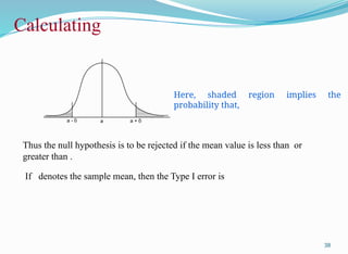
Thus the nullhypothesis is to be rejected if the mean value is less than or
greater than .
If denotes the sample mean, then the Type I error is
38
a - δ a + δ
a
Calculating
Here, shaded region implies the
probability that,
39.
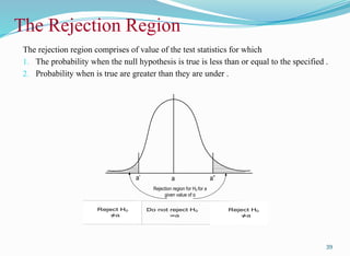
The rejection regioncomprises of value of the test statistics for which
1. The probability when the null hypothesis is true is less than or equal to the specified .
2. Probability when is true are greater than they are under .
39
The Rejection Region
a’ a”
a
Rejection region for H0 for a
given value of α
Reject H0
≠a
Reject H0
≠a
Do not reject H0
=a
40.
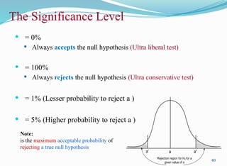
= 0%
Always accepts the null hypothesis (Ultra liberal test)
= 100%
Always rejects the null hypothesis (Ultra conservative test)
= 1% (Lesser probability to reject a )
= 5% (Higher probability to reject a )
40
The Significance Level
a’ a”
a
Rejection region for H0 for a
given value of α
Note:
is the maximum acceptable probability of
rejecting a true null hypothesis
41.
41
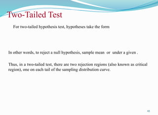
For two-tailed hypothesistest, hypotheses take the form
In other words, to reject a null hypothesis, sample mean or under a given .
Thus, in a two-tailed test, there are two rejection regions (also known as critical
region), one on each tail of the sampling distribution curve.
Two-Tailed Test
42.
42
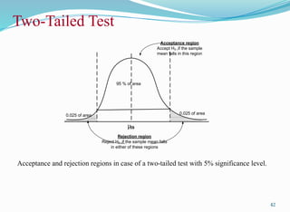
Acceptance and rejectionregions in case of a two-tailed test with 5% significance level.
Two-Tailed Test
µH0
Rejection region
Reject H0 ,if the sample mean falls
in either of these regions
95 % of area
Acceptance region
Accept H0 ,if the sample
mean falls in this region
0.025 of area
0.025 of area
43.
43
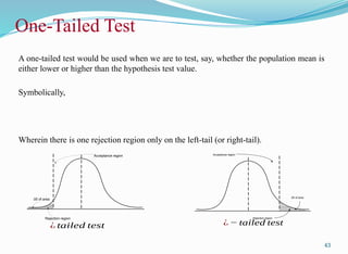
A one-tailed testwould be used when we are to test, say, whether the population mean is
either lower or higher than the hypothesis test value.
Symbolically,
Wherein there is one rejection region only on the left-tail (or right-tail).
One-Tailed Test
Acceptance region
Rejection region
.05 of area
Rejection region
Acceptance region
.05 of area
¿ tailed test ¿ − tailed test
44.
44
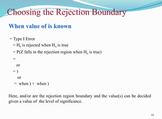
When value ofis known
= Type I Error
= H0 is rejected when H0 is true
= P(Z falls in the rejection region when H0 is true)
=
or
= )
or
= when ) + when )
Here, and/or are the rejection region boundary and the value(s) can be decided
given a value of the level of significance.
Choosing the Rejection Boundary
45.
45
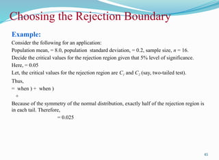
Example:
Consider the followingfor an application:
Population mean, = 8.0, population standard deviation, = 0.2, sample size, n = 16.
Decide the critical values for the rejection region given that 5% level of significance.
Here, = 0.05
Let, the critical values for the rejection region are C1 and C2 (say, two-tailed test).
Thus,
= when ) + when )
+
Because of the symmetry of the normal distribution, exactly half of the rejection region is
in each tail. Therefore,
= 0.025
Choosing the Rejection Boundary
46.
46
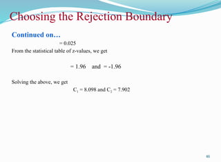
Continued on…
= 0.025
Fromthe statistical table of z-values, we get
= 1.96 and = -1.96
Solving the above, we get
C1 = 8.098 and C2 = 7.902
Choosing the Rejection Boundary
47.
47
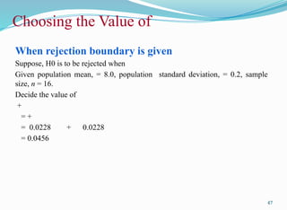
When rejection boundaryis given
Suppose, H0 is to be rejected when
Given population mean, = 8.0, population standard deviation, = 0.2, sample
size, n = 16.
Decide the value of
+
= +
= 0.0228 + 0.0228
= 0.0456
Choosing the Value of
49
The widely usedsampling distribution for parametric tests are
Note:
All these tests are based on the assumption of normality (i.e., the source of data is
considered to be normally distributed).
Parametric Tests and Sampling Distributions
50.
50
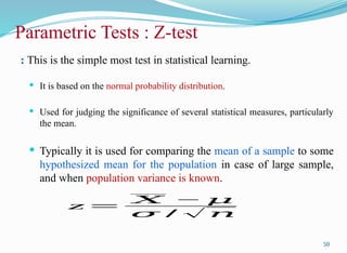
: This isthe simple most test in statistical learning.
It is based on the normal probability distribution.
Used for judging the significance of several statistical measures, particularly
the mean.
Typically it is used for comparing the mean of a sample to some
hypothesized mean for the population in case of large sample,
and when population variance is known.
Parametric Tests : Z-test
z =
𝑋 − 𝜇
𝜎 / √ 𝑛
51.
51
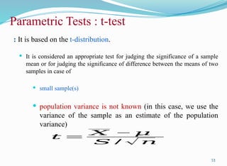
: It isbased on the t-distribution.
It is considered an appropriate test for judging the significance of a sample
mean or for judging the significance of difference between the means of two
samples in case of
small sample(s)
population variance is not known (in this case, we use the
variance of the sample as an estimate of the population
variance)
Parametric Tests : t-test
𝑡 =
𝑋 − 𝜇
𝑆 / √ 𝑛
52.
52
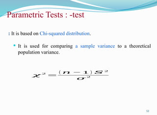
: It isbased on Chi-squared distribution.
It is used for comparing a sample variance to a theoretical
population variance.
Parametric Tests : -test
𝜒
2
=
( 𝑛 − 1 ) 𝑆 2
𝜎 2
55
A coffee vendornearby Nalanda Academic complex has been having average
sales of 500 cups per day. Because of the development of another wing in the
complex, it expects to increase its sales. During the first 12 days, after the
inauguration of the new wing, the daily sales were as under:
550 570 490 615 505 580 570 460 600 580 530 526
On the basis of this sample information, can we conclude that the sales of coffee
have increased?
Consider 5% as the significance level of testing.
Case Study 1: Coffee Sale
56.
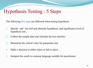
The following fivesteps are followed when testing hypothesis
1. Specify and , the null and alternate hypothesis, and significance level of
hypothesis test .
2. Collect the sample data and calculate the test statistics.
3. Determine the critical value for parametric test.
4. Make a decision to either reject or fail to reject .
5. Interpret the result in common language suitable for practitioner.
56
Hypothesis Testing : 5 Steps
57.
57
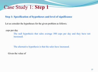
Step 1: Specificationof hypotheses and level of significance
Let us consider the hypotheses for the given problem as follows.
cups per day
The null hypothesis that sales average 500 cups per day and they have not
increased.
The alternative hypothesis is that the sales have increased.
Given the value of
Case Study 1: Step 1
58.
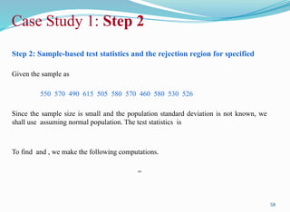
Step 2: Sample-basedtest statistics and the rejection region for specified
Given the sample as
550 570 490 615 505 580 570 460 580 530 526
Since the sample size is small and the population standard deviation is not known, we
shall use assuming normal population. The test statistics is
To find and , we make the following computations.
=
58
Case Study 1: Step 2
61
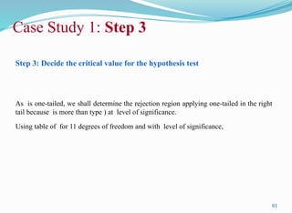
Step 3: Decidethe critical value for the hypothesis test
As is one-tailed, we shall determine the rejection region applying one-tailed in the right
tail because is more than type ) at level of significance.
Using table of for 11 degrees of freedom and with level of significance,
Case Study 1: Step 3
62.
62
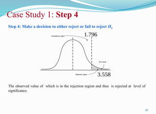
Step 4: Makea decision to either reject or fail to reject H0
The observed value of which is in the rejection region and thus is rejected at level of
significance.
Case Study 1: Step 4
Rejection region
Acceptance region
.05 of area
3.558
1.796
63.
63
Step 5: Finalcomment and interpret the result
We can conclude that the sample data indicate that coffee sales have increased.
Case Study 1: Step 5
64.
64
Step 1: Specificationof hypotheses and significance level
Let us consider the hypotheses for the given problem as follows.
cups per day
The null hypothesis that sales average 500 cups per day and they have not
increased.
The alternative hypothesis is that the sales have increased.
Given the value of
Comments on Case Study 1
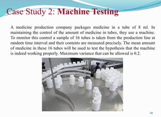
A medicine productioncompany packages medicine in a tube of 8 ml. In
maintaining the control of the amount of medicine in tubes, they use a machine.
To monitor this control a sample of 16 tubes is taken from the production line at
random time interval and their contents are measured precisely. The mean amount
of medicine in these 16 tubes will be used to test the hypothesis that the machine
is indeed working properly. Maximum variance that can be allowed is 0.2.
66
Case Study 2: Machine Testing
67.
Step 1: Specificationof hypothesis and level of significance
The hypotheses are given in terms of the population mean of medicine per tube.
The null hypothesis is
The alternative hypothesis is
We assume , the significance level in our hypothesis testing 0.05.
(This signifies the probability that the machine needs to be adjusted less than 5).
67
Case Study 2: Step 1
68.
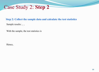
Step 2: Collectthe sample data and calculate the test statistics
Sample results: , ,
With the sample, the test statistics is
Hence,
68
Case Study 2: Step 2
69.
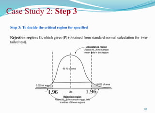
Step 3: Todecide the critical region for specified
Rejection region: G, which gives (P) (obtained from standard normal calculation for two-
tailed test).
69
Case Study 2: Step 3
µH0
Rejection region
Reject H0 ,if the sample mean falls
in either of these regions
95 % of area
Acceptance region
Accept H0 ,if the sample
mean falls in this region
0.025 of area
0.025 of area
1.96
−1.96
70.
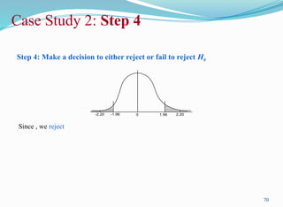
Step 4: Makea decision to either reject or fail to reject H0
Since , we reject
70
-1.96 0
-2.20 1.96 2.20
Case Study 2: Step 4
71.
Step 5: Finalcomment and interpret the result
We conclude and recommend that the machine be adjusted.
71
Case Study 2: Step 5
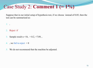
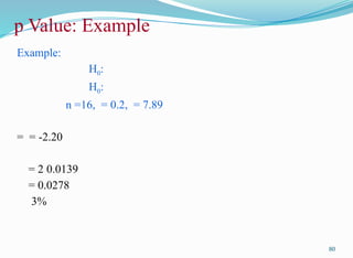
Suppose that inour initial setup of hypothesis test, if we choose instead of 0.05, then the
test can be summarized as:
1. ,
2. Reject if
3. Sample result n =16, = 0.2, =7.89, ,
4. , we fail to reject = 8
5. We do not recommend that the machine be adjusted.
73
Case Study 2: Comment 1 (= 1%)
74.
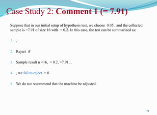
Suppose that inour initial setup of hypothesis test, we choose 0.05, and the collected
sample is =7.91 of size 16 with = 0.2. In this case, the test can be summarized as:
1. ,
2. Reject if
3. Sample result n =16, = 0.2, =7.91, ,
4. , we fail to reject = 8
5. We do not recommend that the machine be adjusted.
74
Case Study 2: Comment 1 (= 7.91)
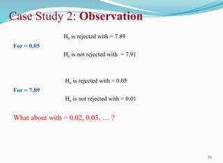
75.
H0 is rejectedwith = 7.89
For = 0.05
H0 is not rejected with = 7.91
H0 is rejected with = 0.05
For = 7.89
H0 is not rejected with = 0.01
What about with = 0.02, 0.03, … ?
75
Case Study 2: Observation
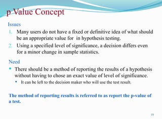
Issues
1. Many usersdo not have a fixed or definitive idea of what should
be an appropriate value for in hypothesis testing.
2. Using a specified level of significance, a decision differs even
for a minor change in sample statistics.
Need
There should be a method of reporting the results of a hypothesis
without having to chose an exact value of level of significance.
It can be left to the decision maker who will use the test result.
The method of reporting results is referred to as report the p-value of
a test.
77
p Value Concept
78.
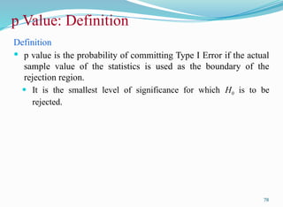
Definition
p valueis the probability of committing Type I Error if the actual
sample value of the statistics is used as the boundary of the
rejection region.
It is the smallest level of significance for which H0 is to be
rejected.
78
p Value: Definition
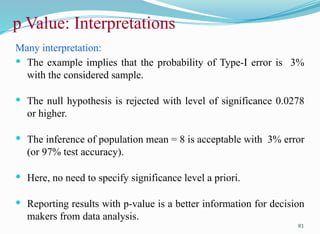
Many interpretation:
Theexample implies that the probability of Type-I error is 3%
with the considered sample.
The null hypothesis is rejected with level of significance 0.0278
or higher.
The inference of population mean = 8 is acceptable with 3% error
(or 97% test accuracy).
Here, no need to specify significance level a priori.
Reporting results with p-value is a better information for decision
makers from data analysis.
81
p Value: Interpretations
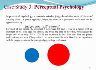
In perceptual psychology,a person is asked to judge the relative areas of circles of
varying sizes. A person typically judges the areas on a perceptual scale that can be
approximated by
For most of the people, the exponent b is between 0.6 and 1. That is a person with an
exponent of 0.8, who sees two circles, one twice the area of the other, would judge the
larger one to be only 20.8
= 1.74. If the exponent is less than one then the person
underestimate the area; if larger than 1, he overestimate the area. Based on an experiment
with 24 people, a data on the perceptual psychology is observed.
83
Case Study 3: Perceptual Psychology
𝐽𝑢𝑑𝑔𝑒𝑑𝑎𝑟𝑒𝑎=𝑎.(𝑇𝑟𝑢𝑒𝑎𝑟𝑒𝑎)𝑏
84.
84
Case Study 3:Perceptual Psychology
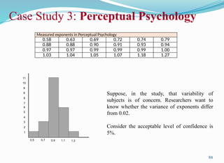
Measured exponents in Perceptual Psychology
0.58 0.63 0.69 0.72 0.74 0.79
0.88 0.88 0.90 0.91 0.93 0.94
0.97 0.97 0.99 0.99 0.99 1.00
1.03 1.04 1.05 1.07 1.18 1.27
Suppose, in the study, that variability of
subjects is of concern. Researchers want to
know whether the variance of exponents differ
from 0.02.
Consider the acceptable level of confidence is
5%.
1
0.5
6
3
2
4
5
7
11
8
8
9
10
0.7 0.9 1.1 1.3
85.
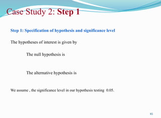
Step 1: Specificationof hypothesis and significance level
The hypotheses of interest is given by
The null hypothesis is
The alternative hypothesis is
We assume , the significance level in our hypothesis testing 0.05.
85
Case Study 2: Step 1
86.
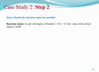
Step 2: Decidethe rejection region for specified
Rejection region: G, and with degree of freedom = 24-1 = 23, the value of the critical
region is 38.08.
86
Case Study 2: Step 2
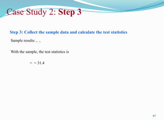
87.
Step 3: Collectthe sample data and calculate the test statistics
Sample results: , ,
With the sample, the test statistics is
= = 31.4
87
Case Study 2: Step 3
88.
Step 4: Makea decision to either reject or fail to reject H0
Since,, we cannot reject the null hypothesis.
88
Case Study 2: Step 4
89.
Step 5: Finalcomment and interpret the result
We conclude that the sample variance does not significantly differ from 0.02.
89
Case Study 2: Step 5
Hypothesis testing issensitive to…
1. , = 10%, 5%, 3%, 2%, 1%, etc.
2. z-test, t-test of -test?
3. Selection of a sample and hence observed values of and S.
4. and repetition of test with different samples.
5. Reporting results with p values without specification of
6. Type-I Error of Type-II Error in testing?
7. ?????.
91
Considerations in Hypothesis Testing
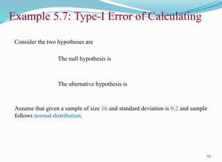
Consider the twohypotheses are
The null hypothesis is
The alternative hypothesis is
Assume that given a sample of size 16 and standard deviation is 0.2 and sample
follows normal distribution.
93
Example 5.7: Type-I Error of Calculating
94.
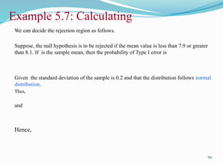
We can decidethe rejection region as follows.
Suppose, the null hypothesis is to be rejected if the mean value is less than 7.9 or greater
than 8.1. If is the sample mean, then the probability of Type I error is
Given the standard deviation of the sample is 0.2 and that the distribution follows normal
distribution.
Thus,
and
Hence,
94
Example 5.7: Calculating
95.
95
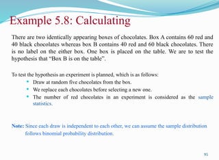
There are twoidentically appearing boxes of chocolates. Box A contains 60 red and
40 black chocolates whereas box B contains 40 red and 60 black chocolates. There
is no label on the either box. One box is placed on the table. We are to test the
hypothesis that “Box B is on the table”.
To test the hypothesis an experiment is planned, which is as follows:
Draw at random five chocolates from the box.
We replace each chocolates before selecting a new one.
The number of red chocolates in an experiment is considered as the sample
statistics.
Note: Since each draw is independent to each other, we can assume the sample distribution
follows binomial probability distribution.
Example 5.8: Calculating
96.
96
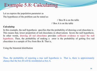
Let us expressthe population parameter as
The hypotheses of the problem can be stated as:
// Box B is on the table
// Box A is on the table
Calculating
In this example, the null hypothesis specifies that the probability of drawing a red chocolate is .
This means that, lower proportion of red chocolates in observations favors the null hypothesis.
In other words, drawing all red chocolates provides sufficient evidence to reject the null
hypothesis. Then, the probability of making a error is the probability of getting five red
chocolates in a sample of five from Box B. That is,
Using the binomial distribution
Thus, the probability of rejecting a true null hypothesis is That is, there is approximately
chance that the box B will be mislabeled as box A.
Example 5.8: Calculating
97.
97
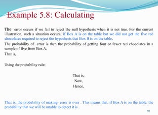
The error occursif we fail to reject the null hypothesis when it is not true. For the current
illustration, such a situation occurs, if Box A is on the table but we did not get the five red
chocolates required to reject the hypothesis that Box B is on the table.
The probability of error is then the probability of getting four or fewer red chocolates in a
sample of five from Box A.
That is,
Using the probability rule:
That is,
Now,
Hence,
That is, the probability of making error is over . This means that, if Box A is on the table, the
probability that we will be unable to detect it is .
Example 5.8: Calculating
99
Estimation
The hypothesistesting makes a statement about the value of a
population parameter. [Subjective estimation]
Instead it may be more interesting to know the value of a population
statistics (e.g., mean score in a quiz rather than if mean = 50 true or
false). [Quantitative estimation]
Such a quantitative estimation in statistical learning is called
estimation (of a population parameter).
100.
100
Estimation
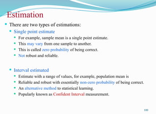
There aretwo types of estimations:
Single point estimate
For example, sample mean is a single point estimate.
This may vary from one sample to another.
This is called zero probability of being correct.
Not robust and reliable.
Interval estimated
Estimate with a range of values, for example, population mean is
Reliable and robust with essentially non-zero probability of being correct.
An alternative method to statistical learning.
Popularly known as Confident Interval measurement.
101.
101
Procedure Confidence IntervalMeasurement
-
=
This implies that
Similarly,
Thus,
< < with probability 1-
Therefore, the interval estimate of is customarily written as
to
102.
102
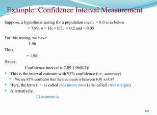
Example: Confidence IntervalMeasurement
Suppose, a hypothesis testing for a population mean = 8.0 is as below.
= 7.89, n = 16, = 0.2, = 0.2 and = 0.05
For this testing, we have
1.96
Thus,
= 1.96
Hence,
Confidence interval is 7.89 1.96(0.2)/
This is the interval estimate with 95% confidence (i.e., accuracy)
We are 95% confident that the true mean is between 6.91 to 8.87
Here, the term E = is called maximum error (also called error margin)
Alternatively,
CI estimate is
104
The hypothesistesting determines the validity of an assumption
(technically described as null hypothesis), with a view to choose
between two conflicting hypothesis about the value of a
population parameter.
There are two types of tests of hypotheses
Parametric tests (also called standard test of hypotheses).
Non-parametric tests (also called distribution-free test of hypotheses).
Hypothesis Testing Strategies
105.
105
Usually assumecertain properties of the population from
which we draw samples.
• Observation come from a normal population
• Sample size is small
• Population parameters like mean, variance, etc. are hold good.
• Requires measurement equivalent to interval scaled data.
Parametric Tests : Applications
106.
106
Case 1: Normalpopulation, population infinite, sample size may be large or small,
variance of the population is known.
Case 2: Population normal, population finite, sample size may large or small………
variance is known.
Case 3: Population normal, population infinite, sample size is small and variance of
the population is unknown.
and
Hypothesis Testing : Assumptions
107.
107
Case 4: Populationis normal, finite, variance is known and sample
with small size
Note:
If variance of population is known, replace by .
Hypothesis Testing
108.
108
Non-Parametric tests
Does not under any assumption
Suitable for nominal or ordinal data
Need entire population (or very large sample size)
Hypothesis Testing : Non-Parametric Test
109.
Reference
109
The detailmaterial related to this lecture can be found in
Probability and Statistics for Engineers and Scientists (8th
Ed.)
by Ronald E. Walpole, Sharon L. Myers, Keying Ye (Pearson),
2013.
110.
Questions of theday…
1. In a hypothesis testing, suppose H0 is rejected. Does it mean that H1 is
accepted? Justify your answer.
2. Give the expressions for z, t and in terms of population and sample
parameters, whichever is applicable to each. Signifies these values in
terms of the respective distributions.
3. How can you obtain the value say P(z = a)? What this values signifies?
4. On what occasion, you should consider z-distribution but not t-
distribution and vice-versa?
5. Give a situation when you should consider distribution but neither z-
nor t-distribution.
110


![99
Estimation
The hypothesis testing makes a statement about the value of a
population parameter. [Subjective estimation]
Instead it may be more interesting to know the value of a population
statistics (e.g., mean score in a quiz rather than if mean = 50 true or
false). [Quantitative estimation]
Such a quantitative estimation in statistical learning is called
estimation (of a population parameter).](https://image.slidesharecdn.com/05statisticallearning-unitii-250215051017-6b4ed481/85/Predictive-analytics-using-R-Programming-99-320.jpg)