Introduction
Inferential statistics havetwo main uses:
• making estimates about populations (for example, the mean
SAT score of all 11th graders in the US).
• testing hypotheses to draw conclusions about populations (for
example, the relationship between SAT scores and family
income).
3.
Introduction
•Setting up andtesting hypotheses is an essential part of
statistical inference. In order to formulate such a test,
usually some theory has been put forward, either
because it is believed to be true or because it is to be
used as a basis for argument, but has not been proved.
•Hypothesis testing refers to the process of using
statistical analysis to determine if the differences
between observed and hypothesized values are due to
random chance or to true differences in the samples.
•Statistical tests separate significant effects from mere
luck or random chance.
•All hypothesis tests have unavoidable but
quantifiable, risks of making the wrong conclusion.
4.
Introduction
•Suppose that apharmaceutical company is concerned that
the mean potency m of an antibiotic to meet the minimum
government potency standards. They need to decide
between two possibilities:
– The mean potency m does not exceed the
required minimum potency.
– The mean potency m exceeds the required
minimum potency.
• This is an example of a test of hypothesis.
5.
Introduction
•Similar to acourtroom trial. To determine a
person committed a crime, the jury needs to
decide between one of two possibilities:
• The person is guilty.
• The person is innocent.
•To begin with, the person is assumed innocent.
•The prosecutor presents evidence, trying to
convince the jury to reject the original
assumption of innocence, and conclude that the
person is guilty.
6.
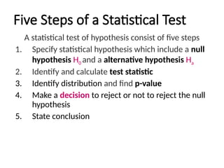
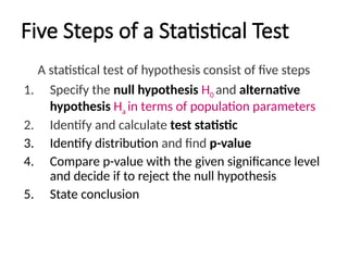
Five Steps ofa Statistical Test
A statistical test of hypothesis consist of five steps
1. Specify statistical hypothesis which include a null
hypothesis H0 and a alternative hypothesis Ha
2. Identify and calculate test statistic
3. Identify distribution and find p-value
4. Make a decision to reject or not to reject the null
hypothesis
5. State conclusion
7.
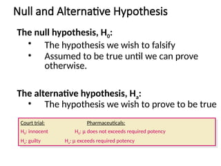
Null and AlternativeHypothesis
The null hypothesis, H0:
• The hypothesis we wish to falsify
• Assumed to be true until we can prove
otherwise.
The alternative hypothesis, Ha:
• The hypothesis we wish to prove to be true
Court trial: Pharmaceuticals:
H0: innocent H0: m does not exceeds required potency
Ha: guilty Ha: m exceeds required potency
8.
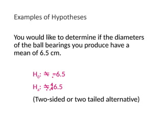
Examples of Hypotheses
Youwould like to determine if the diameters
of the ball bearings you produce have a
mean of 6.5 cm.
H0: =6.5
Ha:
6.5
(Two-sided or two tailed alternative)
9.
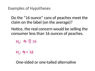
Examples of Hypotheses
Dothe “16 ounce” cans of peaches meet the
claim on the label (on the average)?
Notice, the real concern would be selling the
consumer less than 16 ounces of peaches.
H0: 16
Ha: < 16
One-sided or one-tailed alternative
10.
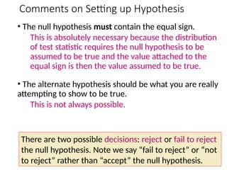
Comments on Settingup Hypothesis
• The null hypothesis must contain the equal sign.
This is absolutely necessary because the distribution
of test statistic requires the null hypothesis to be
assumed to be true and the value attached to the
equal sign is then the value assumed to be true.
• The alternate hypothesis should be what you are really
attempting to show to be true.
This is not always possible.
There are two possible decisions: reject or fail to reject
the null hypothesis. Note we say “fail to reject” or “not
to reject” rather than “accept” the null hypothesis.
11.
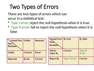
Two Types ofErrors
There are two types of errors which can
occur in a statistical test:
• Type I error: reject the null hypothesis when it is true
• Type II error: fail to reject the null hypothesis when it is
false
Actual Fact
Jury’s
Decision
Guilty Innocent
Guilty Correct Error
Innocent Error Correct
Actual Fact
Your
Decision
H0 true H0 false
Fail to
reject H0
Correct Type II
Error
Reject H0 Type I Error Correct
12.
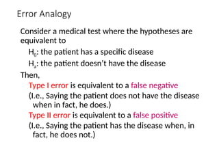
Error Analogy
Consider amedical test where the hypotheses are
equivalent to
H0: the patient has a specific disease
Ha: the patient doesn’t have the disease
Then,
Type I error is equivalent to a false negative
(I.e., Saying the patient does not have the disease
when in fact, he does.)
Type II error is equivalent to a false positive
(I.e., Saying the patient has the disease when, in
fact, he does not.)
13.
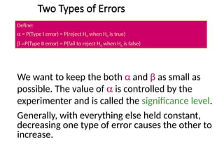
Two Types ofErrors
We want to keep the both α and β as small as
possible. The value of a is controlled by the
experimenter and is called the significance level.
Generally, with everything else held constant,
decreasing one type of error causes the other to
increase.
Define:
a = P(Type I error) = P(reject H0 when H0 is true)
b =P(Type II error) = P(fail to reject H0 when H0 is false)
14.
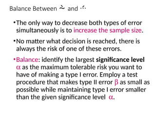
Balance Between and
•The only way to decrease both types of error
simultaneously is to increase the sample size.
•No matter what decision is reached, there is
always the risk of one of these errors.
•Balance: identify the largest significance level
a as the maximum tolerable risk you want to
have of making a type I error. Employ a test
procedure that makes type II error b as small as
possible while maintaining type I error smaller
than the given significance level a.
15.
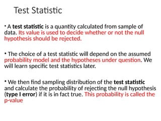
Test Statistic
• Atest statistic is a quantity calculated from sample of
data. Its value is used to decide whether or not the null
hypothesis should be rejected.
• The choice of a test statistic will depend on the assumed
probability model and the hypotheses under question. We
will learn specific test statistics later.
• We then find sampling distribution of the test statistic
and calculate the probability of rejecting the null hypothesis
(type I error) if it is in fact true. This probability is called the
p-value
16.
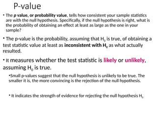
P-value
• The pvalue, or probability value, tells how consistent your sample statistics
are with the null hypothesis. Specifically, if the null hypothesis is right, what is
the probability of obtaining an effect at least as large as the one in your
sample?
• The p-value is the probability, assuming that H0 is true, of obtaining a
test statistic value at least as inconsistent with H0 as what actually
resulted.
• It measures whether the test statistic is likely or unlikely,
assuming H0 is true.
•Small p-values suggest that the null hypothesis is unlikely to be true. The
smaller it is, the more convincing is the rejection of the null hypothesis.
• It indicates the strength of evidence for rejecting the null hypothesis H0
17.
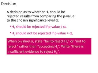
Decision
A decision asto whether H0 should be
rejected results from comparing the p-value
to the chosen significance level a:
•H0 should be rejected if p-value a.
•H0 should not be rejected if p-value > a.
When p-value>α, state “fail to reject H0” or “not to
reject” rather than “accepting H0”. Write “there is
insufficient evidence to reject H0”.
18.
Five Steps ofa Statistical Test
A statistical test of hypothesis consist of five steps
1. Specify the null hypothesis H0 and alternative
hypothesis Ha in terms of population parameters
2. Identify and calculate test statistic
3. Identify distribution and find p-value
4. Compare p-value with the given significance level
and decide if to reject the null hypothesis
5. State conclusion
19.
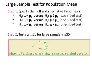
Large Sample Testfor Population Mean
Step 1: Specify the null and alternative hypothesis
• H0: m = m0 versus Ha: m m0 (two-sided test)
• H0: m = m0 versus Ha: m > m0 (one-sided test)
• H0: m = m0 versus Ha: m < m0 (one-sided test)
Step 2: Test statistic for large sample (n≥30)
deviation
standard
and
mean
size,
sample
are
s
and
n,
where
/
0
x
n
s
x
z
20.
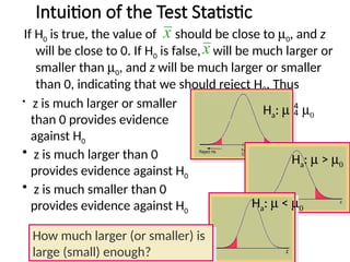
Intuition of theTest Statistic
If H0 is true, the value of should be close to m0, and z
will be close to 0. If H0 is false, will be much larger or
smaller than m0, and z will be much larger or smaller
than 0, indicating that we should reject H0. Thus
x
x
Ha: m m0
Ha: m > m0
Ha: m < m0
• z is much larger or smaller
than 0 provides evidence
against H0
• z is much larger than 0
provides evidence against H0
• z is much smaller than 0
provides evidence against H0
How much larger (or smaller) is
large (small) enough?
21.
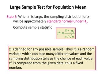
Large Sample Testfor Population Mean
Step 3: When n is large, the sampling distribution of z
will be approximately standard normal under H0.
Compute sample statistic
n
s
x
z
/
* 0
z is defined for any possible sample. Thus it is a random
variable which can take many different values and the
sampling distribution tells us the chance of each value.
z* is computed from the given data, thus a fixed
number.
22.
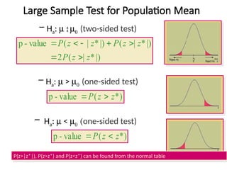
Large Sample Testfor Population Mean
– Ha: m < m0 (one-sided test)
*)
(
value
-
p z
z
P
– Ha: m > m0 (one-sided test)
*)
(
value
-
p z
z
P
|)
*
|
(
2
|)
*
|
(
|)
*
|
(
value
-
p
z
z
P
z
z
P
z
z
P
– Ha: m m0 (two-sided test)
P(z>|z*|), P(z>z*) and P(z<z*) can be found from the normal table
23.
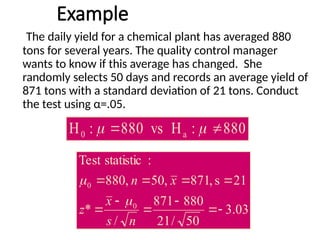
Example
The daily yieldfor a chemical plant has averaged 880
tons for several years. The quality control manager
wants to know if this average has changed. She
randomly selects 50 days and records an average yield of
871 tons with a standard deviation of 21 tons. Conduct
the test using α=.05.
880
:
H
vs
880
:
H a
0
03
.
3
50
/
21
880
871
/
*
21
s
,
871
,
50
,
880
:
statistic
Test
0
0
n
s
x
z
x
n
24.
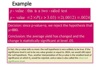
Example
0024
.
)
0012
(.
2
)
03
.
3
(
2
value
test
sided
-
two
a
is
this
:
value
-
z
P
p
p
Decision: sincep-value<α, we reject the hypothesis that
μ=880.
Conclusion: the average yield has changed and the
change is statistically significant at level .05.
In fact, the p-value tells us more: the null hypothesis is very unlikely to be true. If the
significance level is set to be any value greater or equal to .0024, we would still reject
the null hypothesis. Thus, another interpretation of the p-value is the smallest level of
significance at which H0 would be rejected, and p-value is also called the observed
significance level.
25.
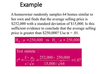
Example
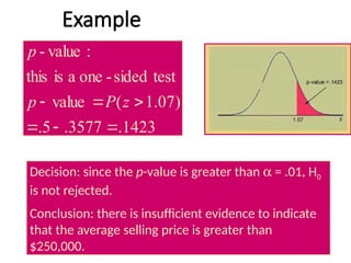
A homeowner randomlysamples 64 homes similar to
her own and finds that the average selling price is
$252,000 with a standard deviation of $15,000. Is this
sufficient evidence to conclude that the average selling
price is greater than $250,000? Use a = .01.
000
,
250
:
H
vs
000
,
250
:
H a
0
07
.
1
64
/
000
,
15
000
,
250
000
,
252
/
*
:
statistic
Test
0
n
s
x
z
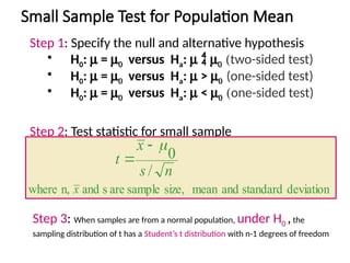
Small Sample Testfor Population Mean
Step 1: Specify the null and alternative hypothesis
• H0: m = m0 versus Ha: m m0 (two-sided test)
• H0: m = m0 versus Ha: m > m0 (one-sided test)
• H0: m = m0 versus Ha: m < m0 (one-sided test)
Step 2: Test statistic for small sample
deviation
standard
and
mean
size,
sample
are
s
and
n,
where
/
0
x
n
s
x
t
Step 3: When samples are from a normal population, under H0 ,the
sampling distribution of t has a Student’s t distribution with n-1 degrees of freedom
28.
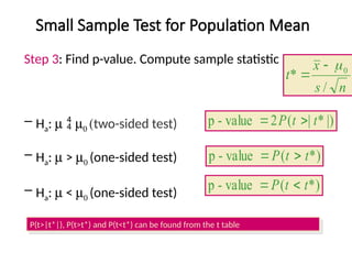
Small Sample Testfor Population Mean
Step 3: Find p-value. Compute sample statistic
n
s
x
t
/
* 0
– Ha: m m0 (two-sided test)
– Ha: m > m0 (one-sided test)
– Ha: m < m0 (one-sided test)
|)
*
|
(
2
value
-
p t
t
P
*)
(
value
-
p t
t
P
*)
(
value
-
p t
t
P
P(t>|t*|), P(t>t*) and P(t<t*) can be found from the t table
29.
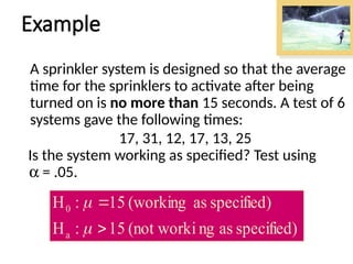
Example
A sprinkler systemis designed so that the average
time for the sprinklers to activate after being
turned on is no more than 15 seconds. A test of 6
systems gave the following times:
17, 31, 12, 17, 13, 25
Is the system working as specified? Test using
a = .05.
specified)
as
ng
(not worki
15
:
H
specified)
as
(working
15
:
H
a
0
30.
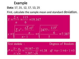
Example
Data: 17, 31,12, 17, 13, 25
First, calculate the sample mean and standard deviation.
387
.
7
5
6
115
2477
1
)
(
167
.
19
6
115
2
2
2
n
n
x
x
s
n
x
x i
5
1
6
1
38
.
1
6
/
387
.
7
15
167
.
19
/
*
:
freedom
of
Degrees
:
statistic
Test
0
n
df
n
s
x
t
31.
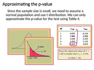
Approximating the p-value
Sincethe sample size is small, we need to assume a
normal population and use t distribution. We can only
approximate the p-value for the test using Table 4.
Since the observed value of t* =
1.38 is smaller than t.10 = 1.476,
p-value > .10.
32.
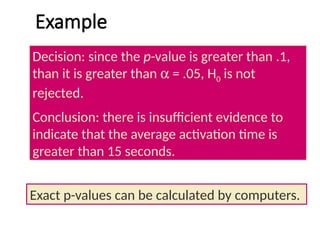
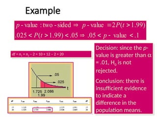
Example
Decision: since thep-value is greater than .1,
than it is greater than a = .05, H0 is not
rejected.
Conclusion: there is insufficient evidence to
indicate that the average activation time is
greater than 15 seconds.
Exact p-values can be calculated by computers.
33.
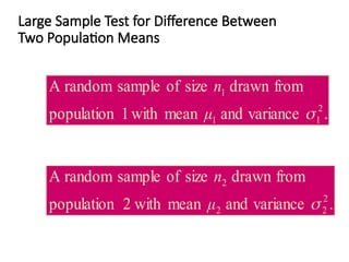
Large Sample Testfor Difference Between
Two Population Means
.
variance
and
mean
with
1
population
from
drawn
size
of
sample
random
A
2
1
1
1
μ
n
.
variance
and
mean
with
2
population
from
drawn
size
of
sample
random
A
2
2
2
2
μ
n
34.
Large Sample Testfor Difference Between
Two Population Means
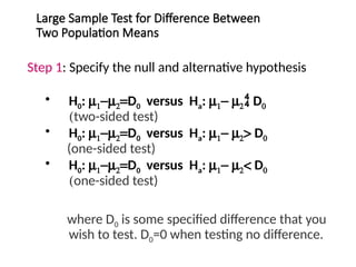
Step 1: Specify the null and alternative hypothesis
• H0: m1-m2=D0 versus Ha: m1- m2 D0
(two-sided test)
• H0: m1-m2=D0 versus Ha: m1- m2> D0
(one-sided test)
• H0: m1-m2=D0 versus Ha: m1- m2< D0
(one-sided test)
where D0 is some specified difference that you
wish to test. D0=0 when testing no difference.
35.
Large Sample Testfor Difference Between
Two Population Means
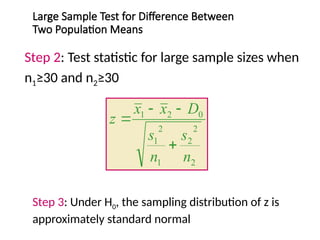
Step 2: Test statistic for large sample sizes when
n1≥30 and n2≥30
2
2
2
1
2
1
0
2
1
n
s
n
s
D
x
x
z
Step 3: Under H0, the sampling distribution of z is
approximately standard normal
36.
Large Sample Testfor Difference Between
Two Population Means
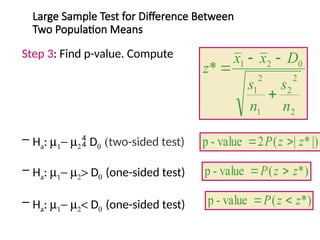
Step 3: Find p-value. Compute
– Ha: m1- m2 D0 (two-sided test)
– Ha: m1- m2> D0 (one-sided test)
– Ha: m1- m2< D0 (one-sided test)
|)
*
|
(
2
value
-
p z
z
P
2
2
2
1
2
1
0
2
1
*
n
s
n
s
D
x
x
z
*)
(
value
-
p z
z
P
*)
(
value
-
p z
z
P
37.
Example
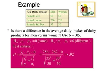
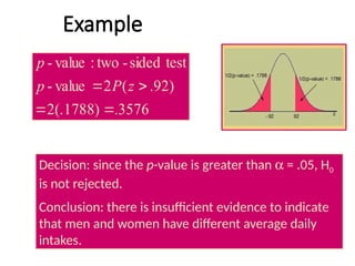
• Is therea difference in the average daily intakes of dairy
products for men versus women? Use a = .05.
Avg Daily Intakes Men Women
Sample size 50 50
Sample mean 756 762
Sample Std Dev 35 30
(same)
0
:
H 2
1
0
2
2
2
1
2
1
2
1 0
*
:
statistic
Test
n
s
n
s
x
x
z
)
(different
0
:
H 2
1
a
92
.
50
30
50
35
0
762
756
2
2
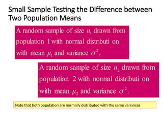
Small Sample Testingthe Difference between
Two Population Means
.
variance
and
mean
with
on
distributi
normal
with
1
population
from
drawn
size
of
sample
random
A
2
1
1
μ
n
.
variance
and
mean
with
on
distributi
normal
with
2
population
from
drawn
size
of
sample
random
A
2
2
2
μ
n
Note that both population are normally distributed with the same variances
40.
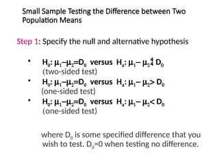
Small Sample Testingthe Difference between Two
Population Means
Step 1: Specify the null and alternative hypothesis
• H0: m1-m2=D0 versus Ha: m1- m2 D0
(two-sided test)
• H0: m1-m2=D0 versus Ha: m1- m2> D0
(one-sided test)
• H0: m1-m2=D0 versus Ha: m1- m2< D0
(one-sided test)
where D0 is some specified difference that you
wish to test. D0=0 when testing no difference.
41.
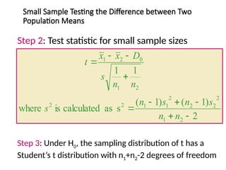
Small Sample Testingthe Difference between Two
Population Means
Step 2: Test statistic for small sample sizes
2
)
1
(
)
1
(
s
as
calculated
is
where
1
1
2
1
2
2
2
2
1
1
2
2
2
1
0
2
1
n
n
s
n
s
n
s
n
n
s
D
x
x
t
Step 3: Under H0, the sampling distribution of t has a
Student’s t distribution with n1+n2-2 degrees of freedom
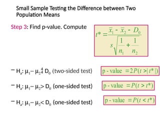
42.
Small Sample Testingthe Difference between Two
Population Means
Step 3: Find p-value. Compute
– Ha: m1- m2 D0 (two-sided test)
– Ha: m1- m2> D0 (one-sided test)
– Ha: m1- m2< D0 (one-sided test)
|)
*
|
(
2
value
-
p t
t
P
*)
(
value
-
p t
t
P
*)
(
value
-
p t
t
P
1
1
*
2
1
0
2
1
n
n
s
D
x
x
t
43.
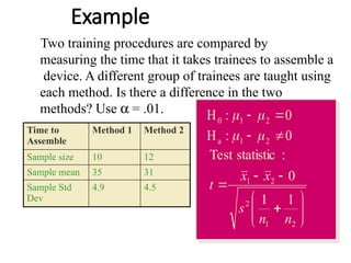
Example
Two training proceduresare compared by
measuring the time that it takes trainees to assemble a
device. A different group of trainees are taught using
each method. Is there a difference in the two
methods? Use a = .01.
Time to
Assemble
Method 1 Method 2
Sample size 10 12
Sample mean 35 31
Sample Std
Dev
4.9 4.5
0
:
H 2
1
0
2
1
2
2
1
1
1
0
:
statistic
Test
n
n
s
x
x
t
0
:
H 2
1
a
44.
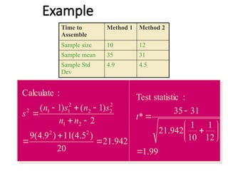
Example
Time to
Assemble
Method 1Method 2
Sample size 10 12
Sample mean 35 31
Sample Std
Dev
4.9 4.5
99
.
1
12
1
10
1
942
.
21
31
35
*
:
statistic
Test
t
942
.
21
20
)
5
.
4
(
11
)
9
.
4
(
9
2
)
1
(
)
1
(
:
Calculate
2
2
2
1
2
2
2
2
1
1
2
n
n
s
n
s
n
s
Key Concepts
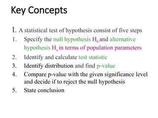
I. Astatistical test of hypothesis consist of five steps
1. Specify the null hypothesis H0 and alternative
hypothesis Ha in terms of population parameters
2. Identify and calculate test statistic
3. Identify distribution and find p-value
4. Compare p-value with the given significance level
and decide if to reject the null hypothesis
5. State conclusion
47.
Key Concepts
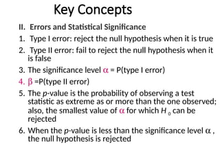
II. Errorsand Statistical Significance
1. Type I error: reject the null hypothesis when it is true
2. Type II error: fail to reject the null hypothesis when it
is false
3. The significance level a = P(type I error)
4. b =P(type II error)
5. The p-value is the probability of observing a test
statistic as extreme as or more than the one observed;
also, the smallest value of a for which H 0 can be
rejected
6. When the p-value is less than the significance level a ,
the null hypothesis is rejected
48.
Key Concepts
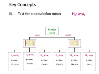
III. Testfor a population mean H0: µ=µ0
n
s
x
z
/
0
Sample
size?
Ha: µ≠µ0
p-value=
2P(z>|z*|)
Ha: µ>µ0
p-value=
P(z>z*)
Ha: µ<µ0
p-value=
P(z<z*)
Ha: µ≠µ0
p-value=
2P(t>|t*|)
Ha: µ>µ0
p-value=
2P(t>t*)
Ha: µ≠µ0
p-value=
P(t<t*)
n
s
x
t
/
0
large small
49.
Key Concepts
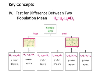
IV. Testfor Difference Between Two
Population Mean H0: µ1-µ2=D0
Sample
size?
Ha: µ1-µ2≠D0
p-value=
2P(z>|z*|)
Ha: µ1-µ2>D0
p-value=
P(z>z*)
Ha: µ1-µ2<D0
p-value=
P(z<z*)
Ha:µ1-µ2≠D0
p-value=
2P(t>|t*|)
Ha: µ1-µ2>D0
p-value=
2P(t>t*)
Ha: µ1-µ2<D0
p-value=
P(t<t*)
large small
2
2
2
1
2
1
0
2
1
n
s
n
s
D
x
x
z
2
1
0
2
1
1
1
n
n
s
D
x
x
t
50.
• To trustyour model and make predictions,
we utilize hypothesis testing. When we will
use sample data to train our model, we
make assumptions about our population.
• By performing hypothesis testing, we
validate these assumptions for a desired
significance level.