Downloaded 527 times
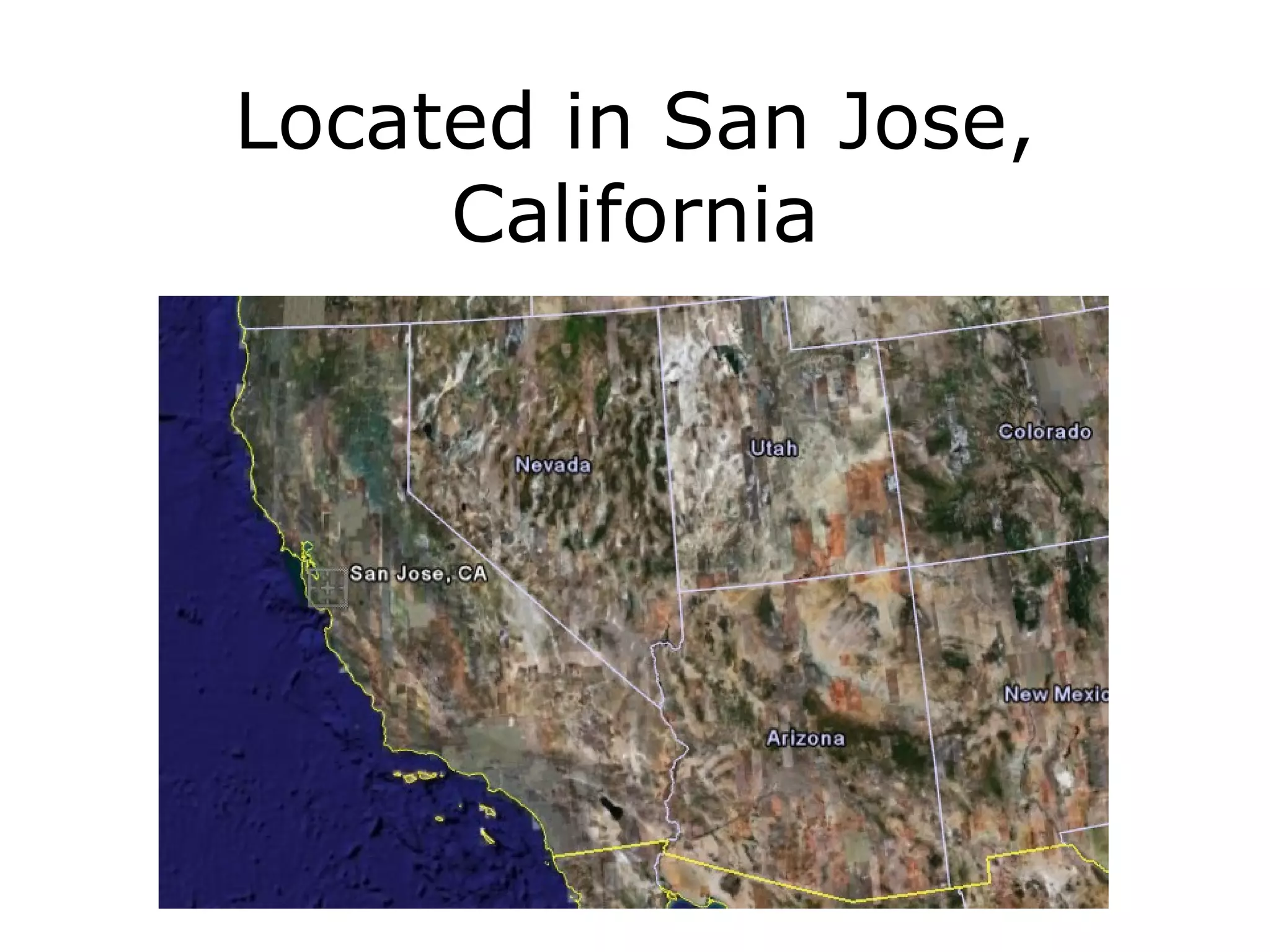
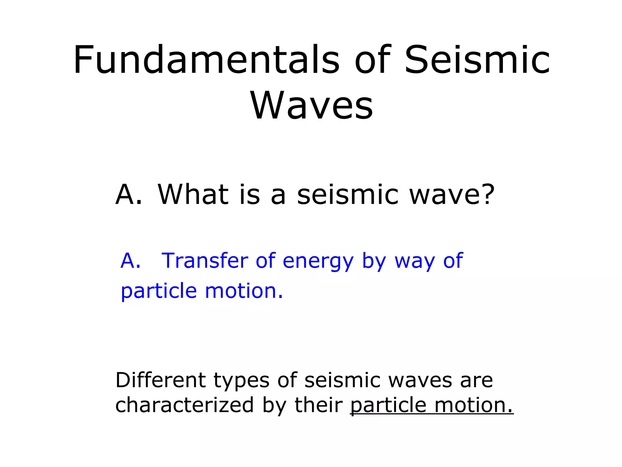
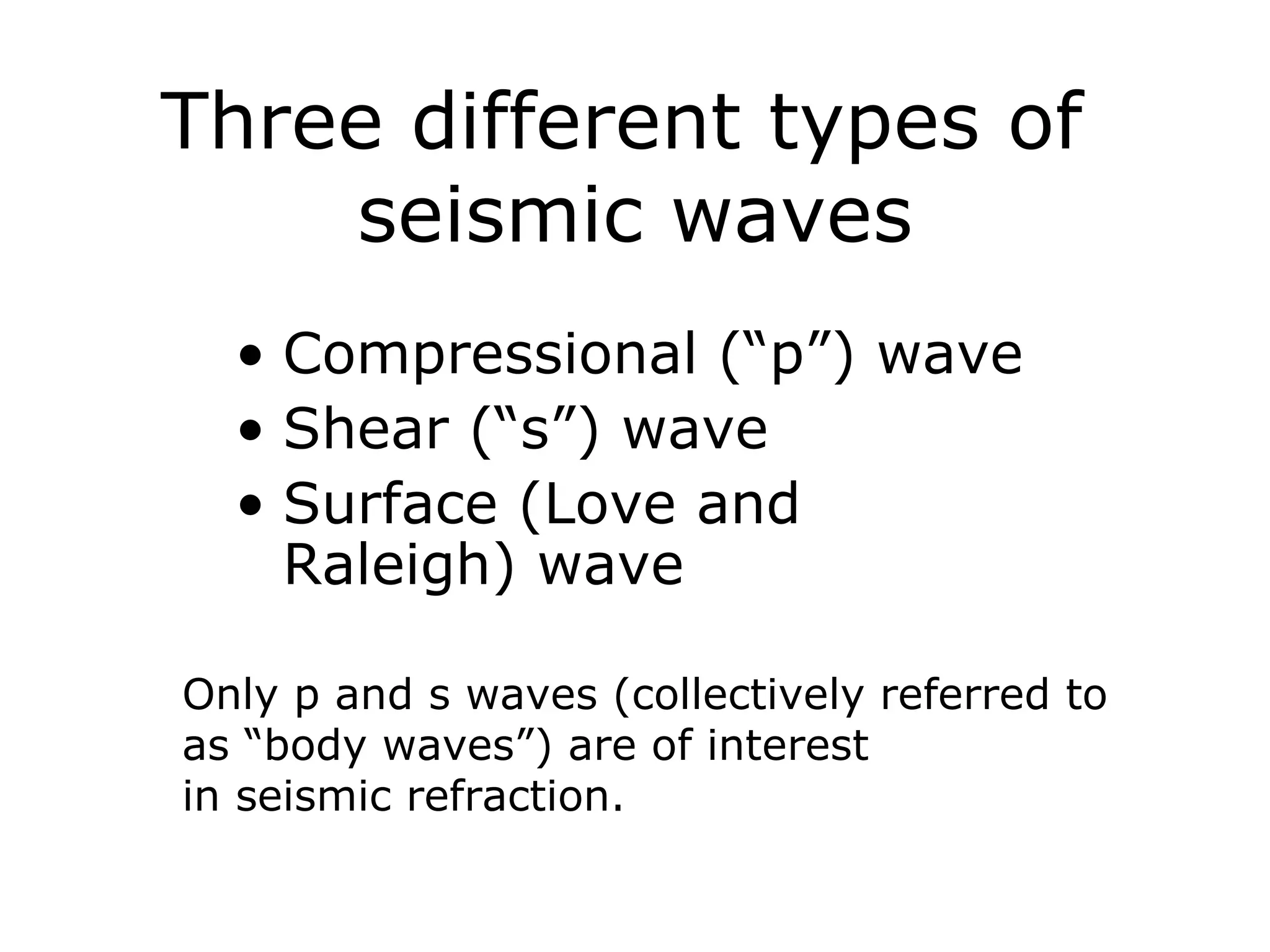
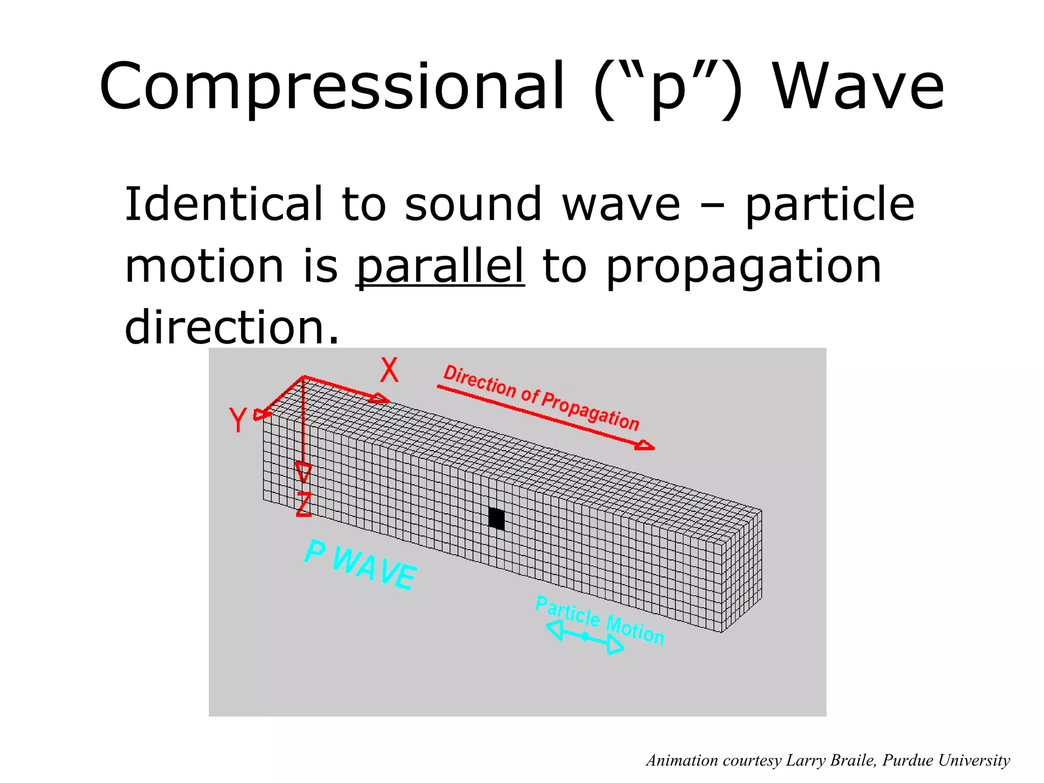
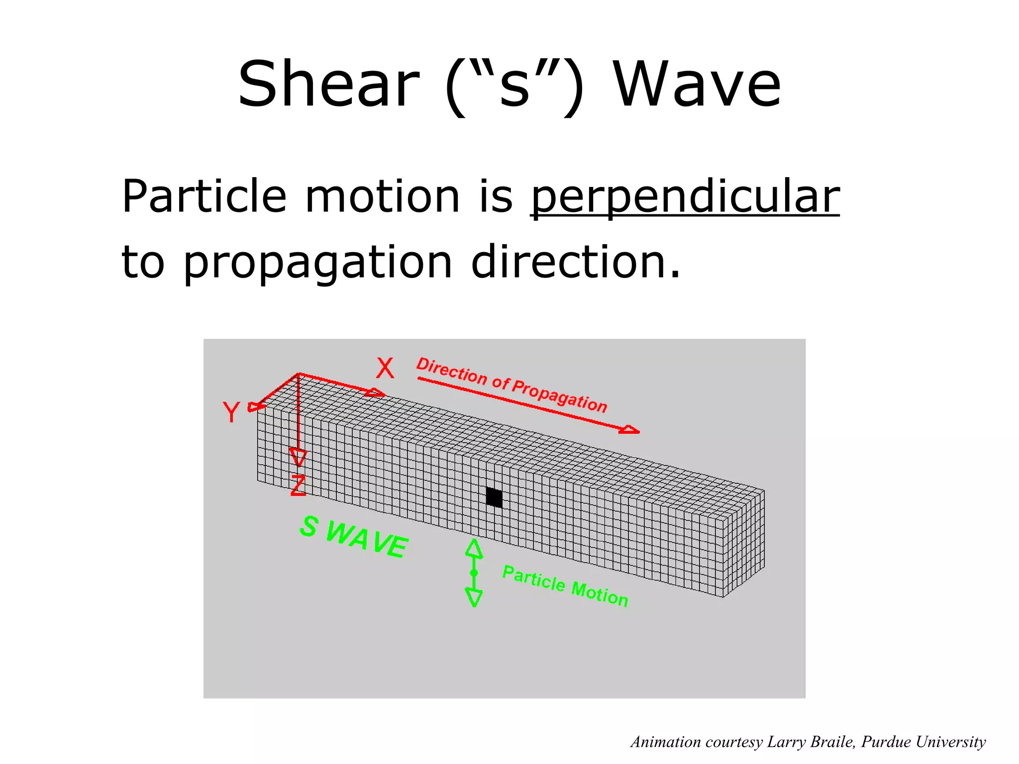
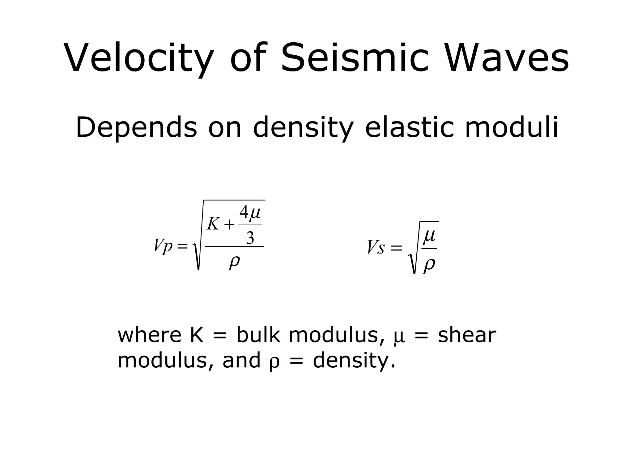
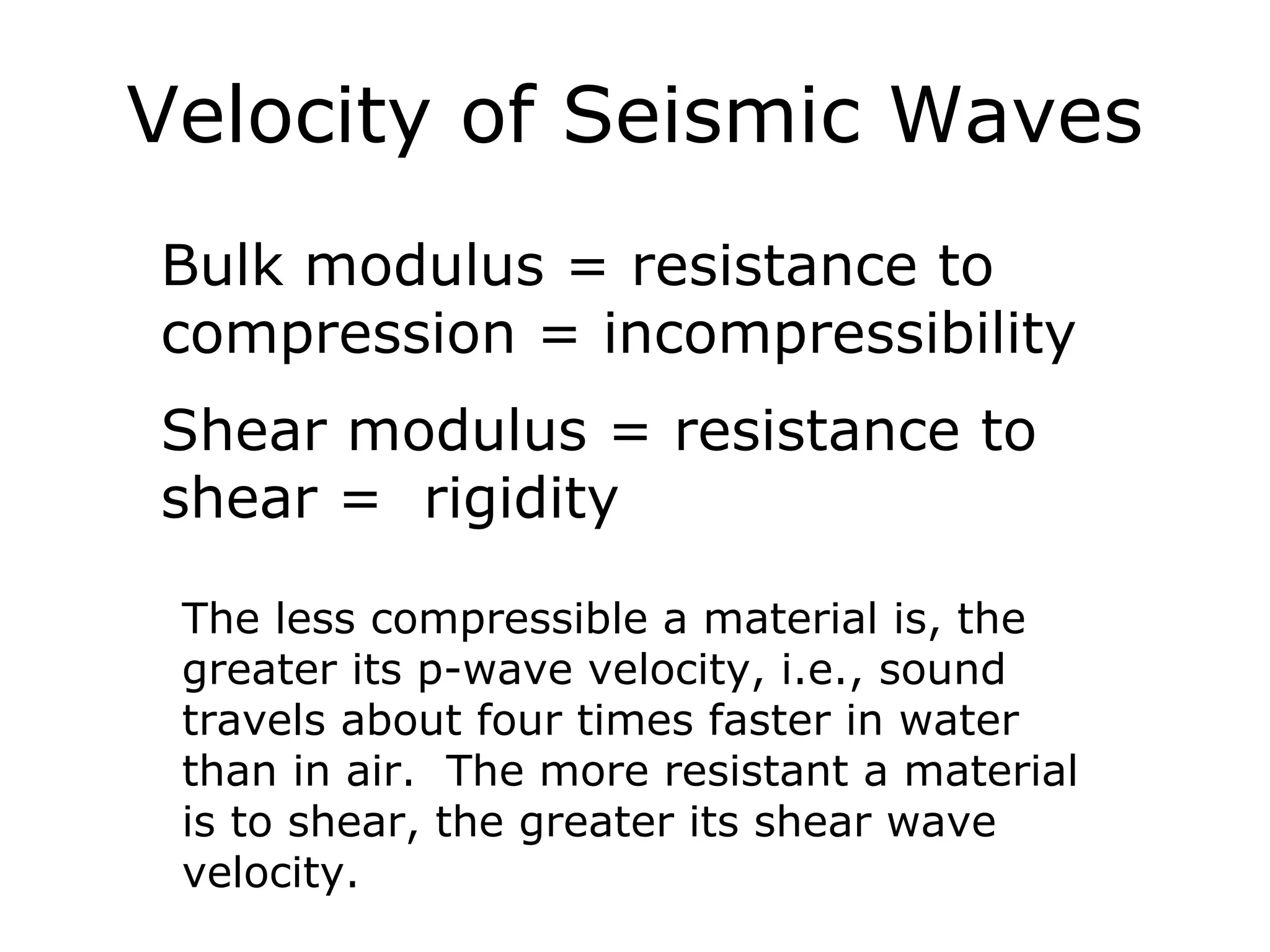
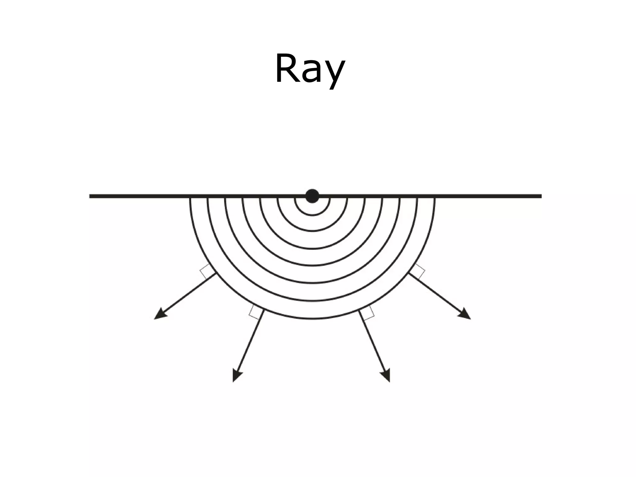
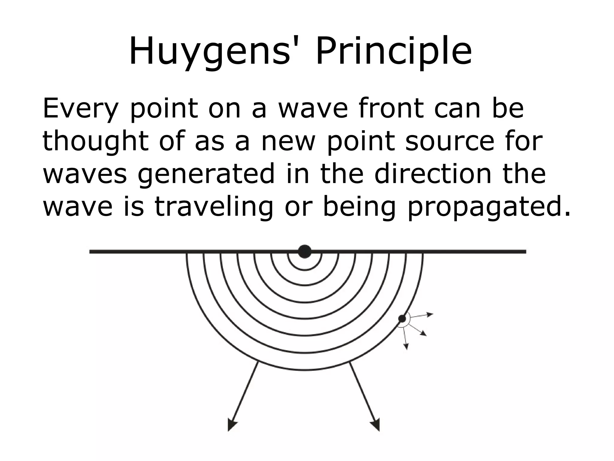
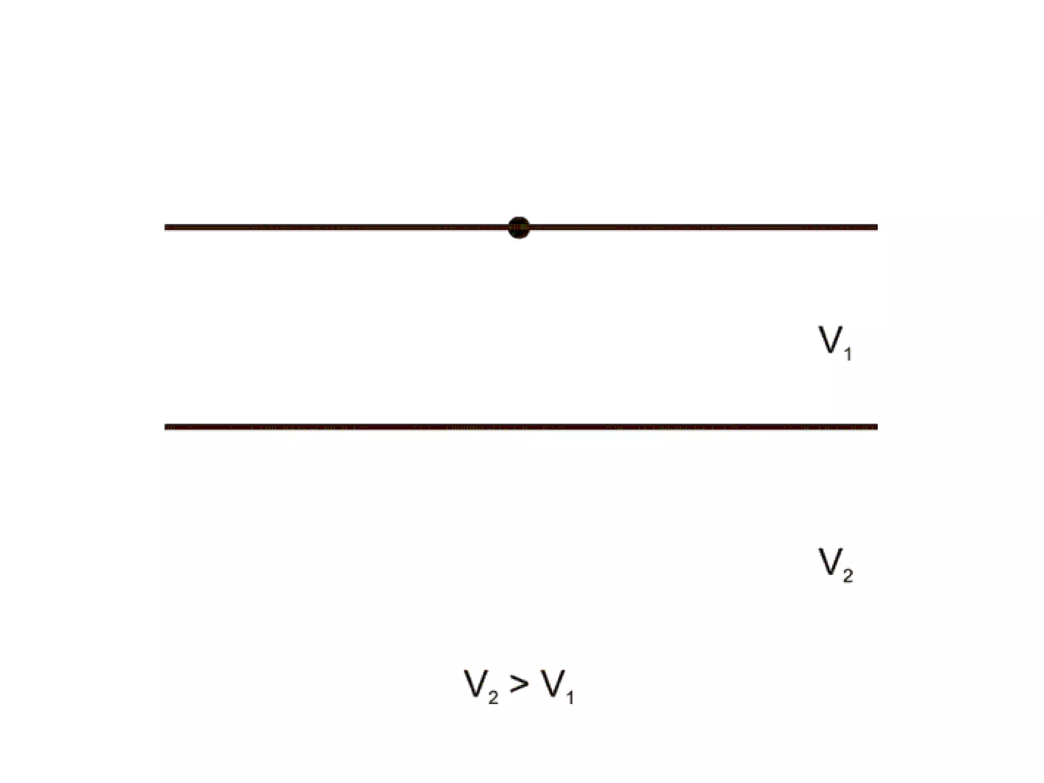
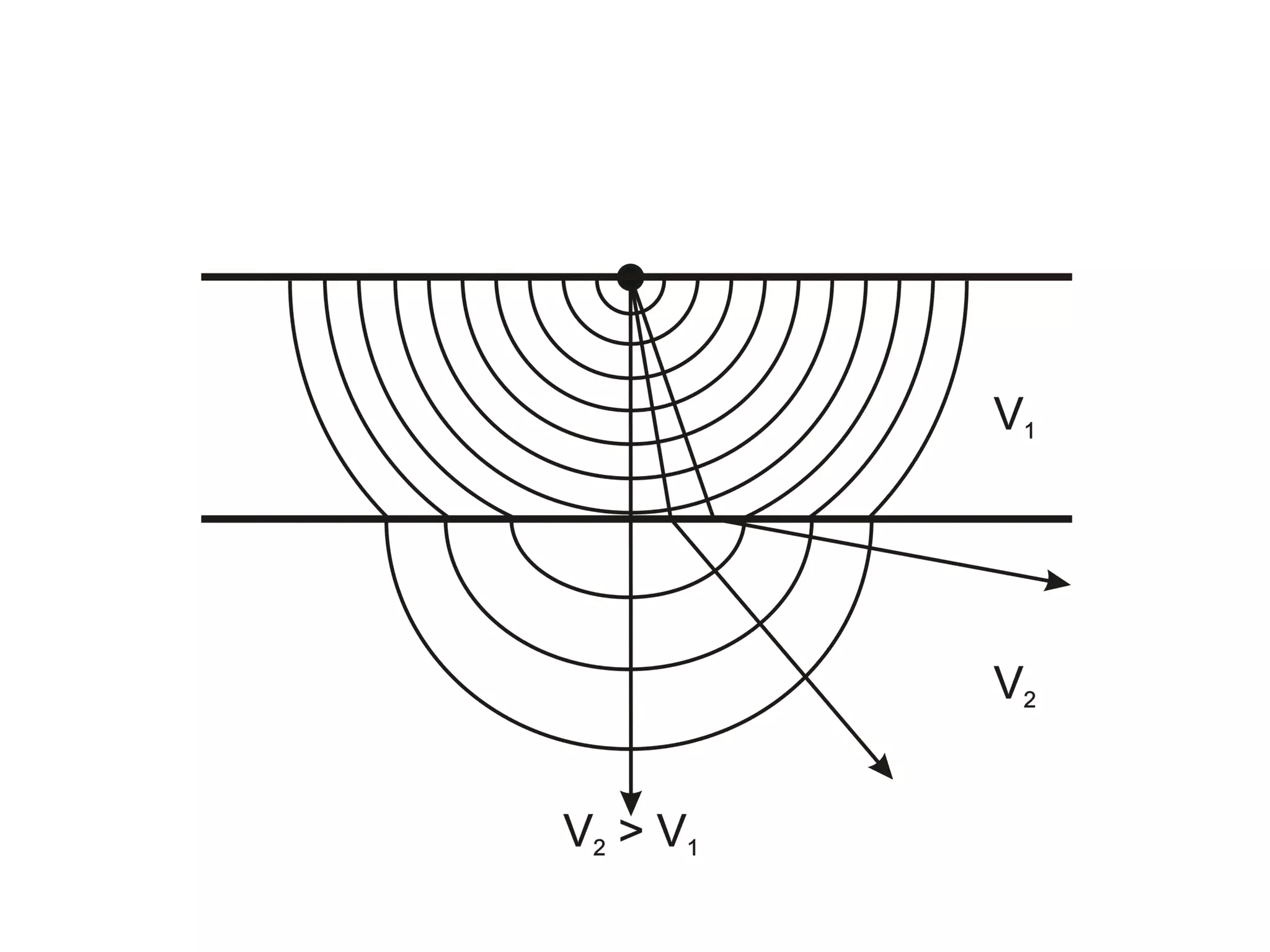
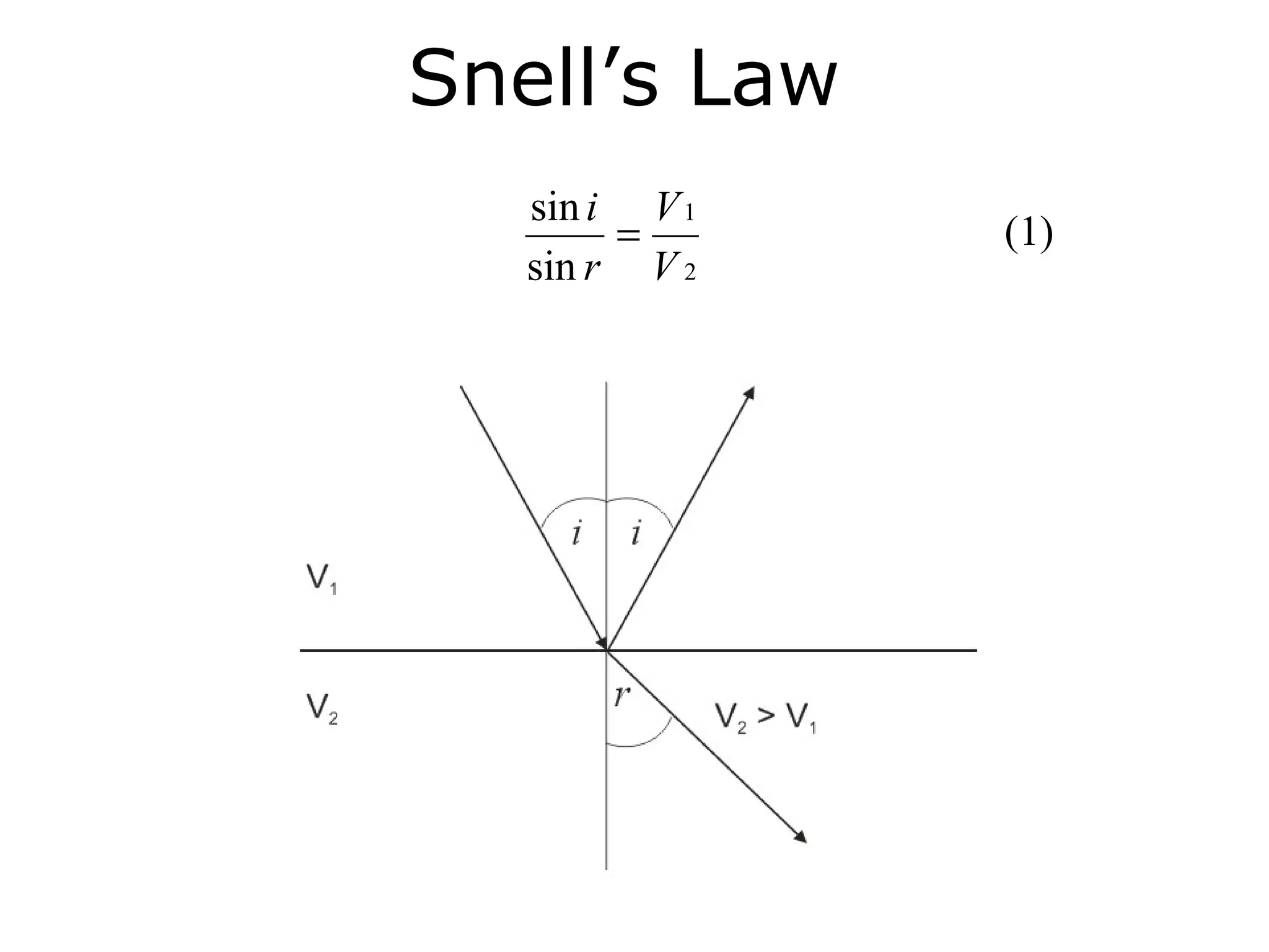
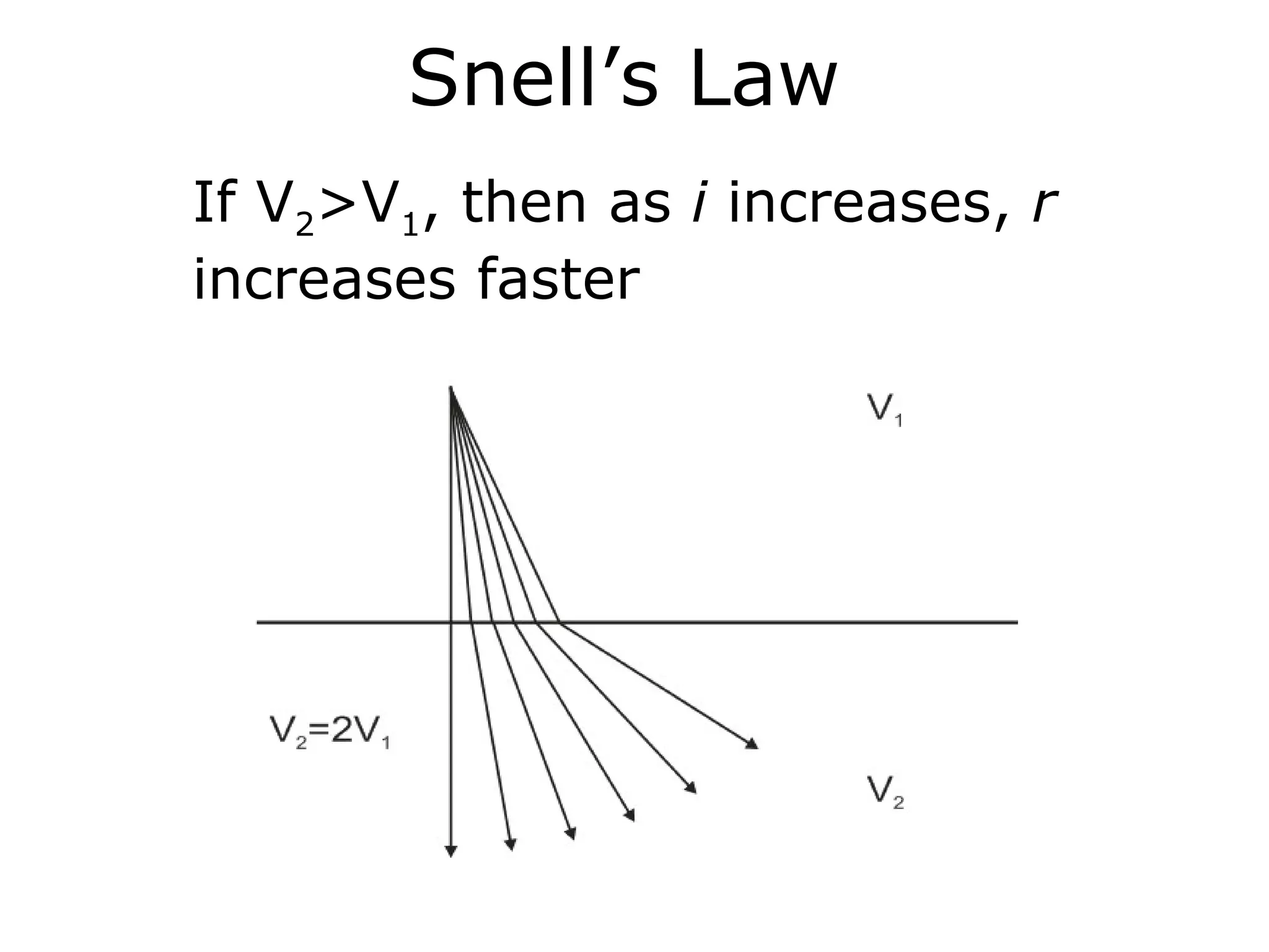
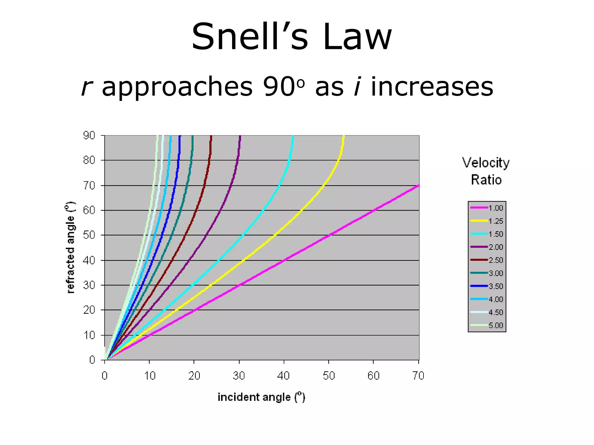
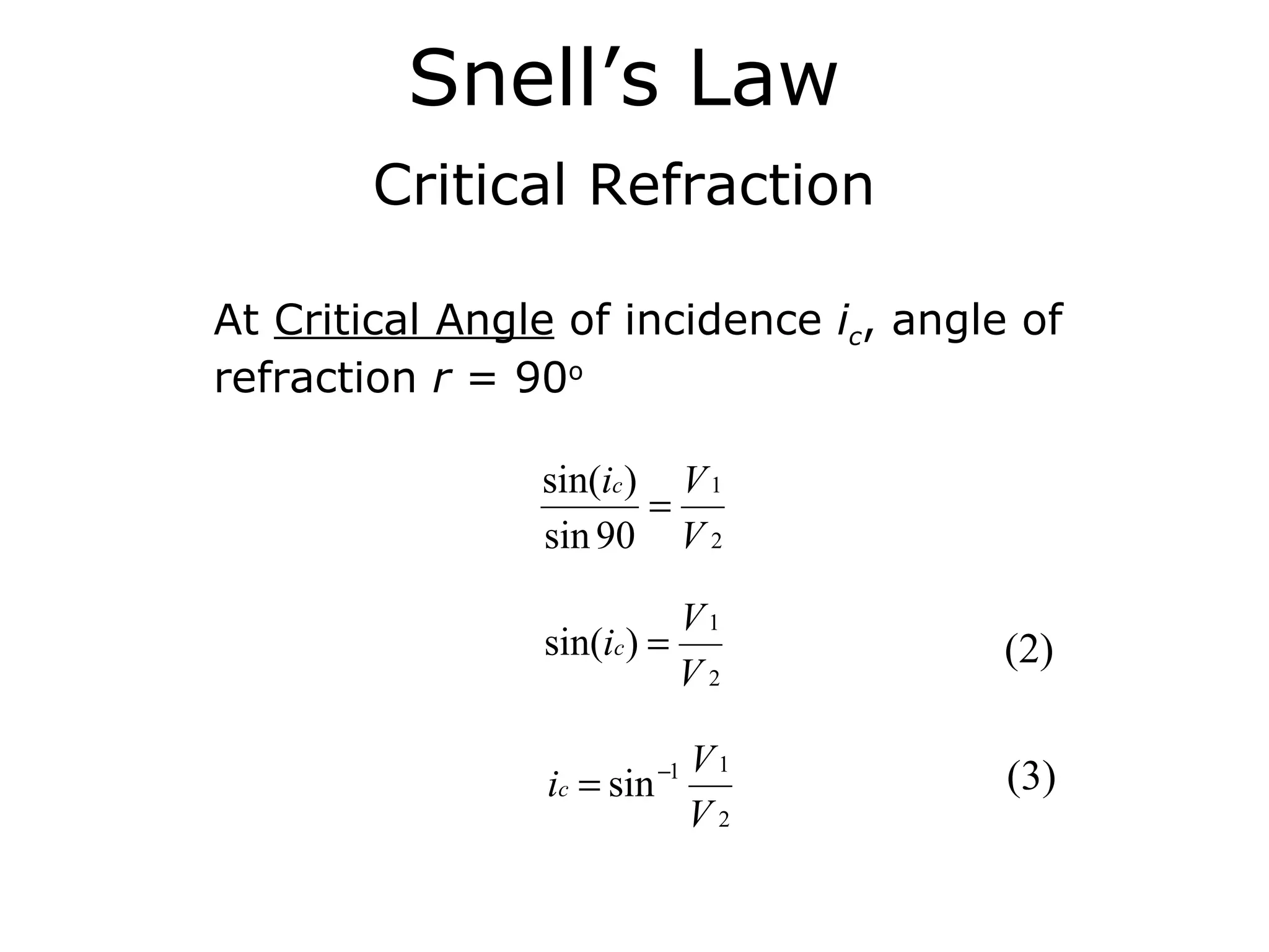
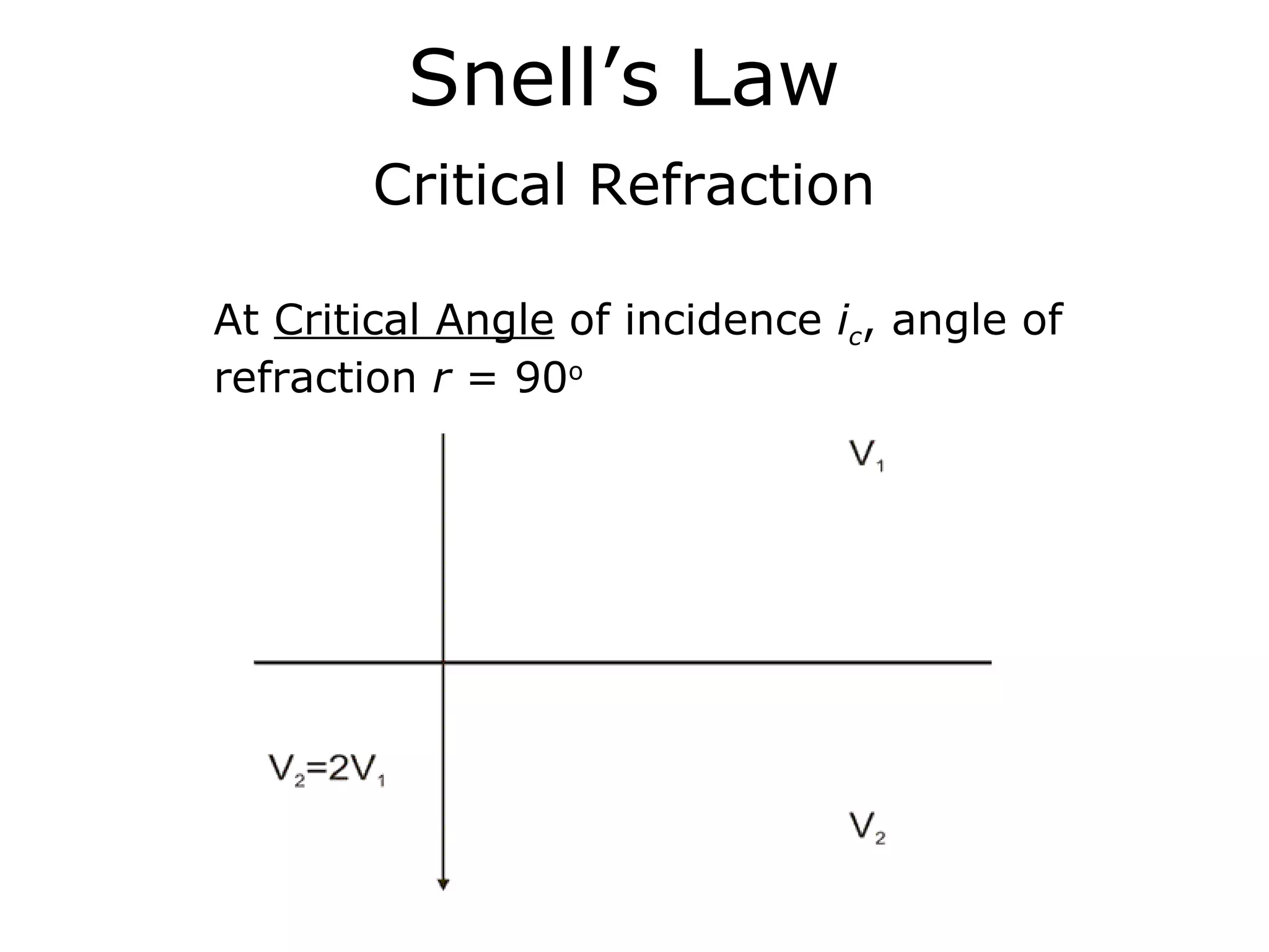
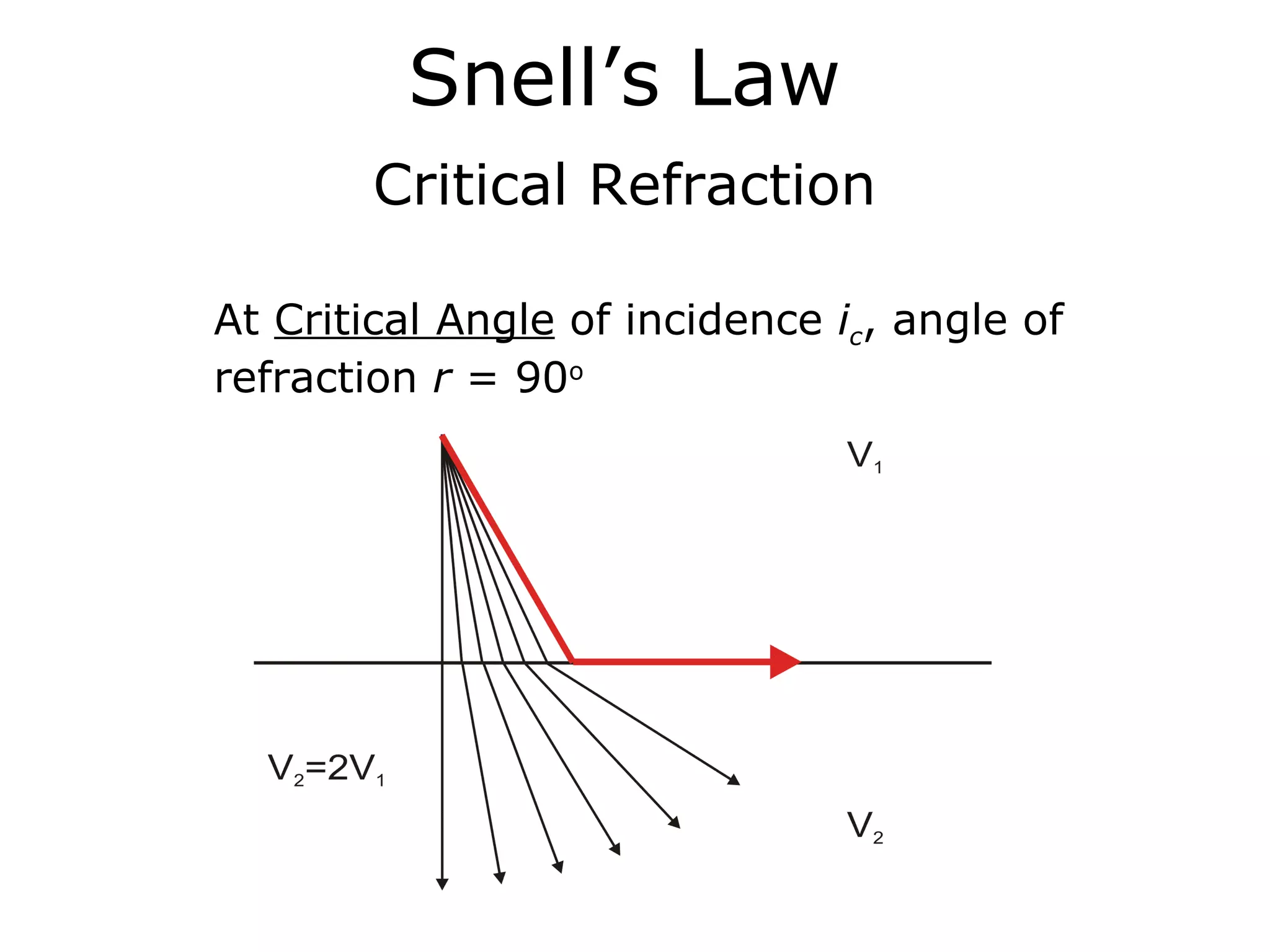
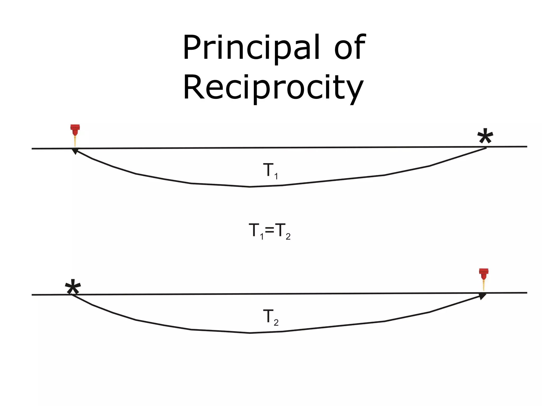
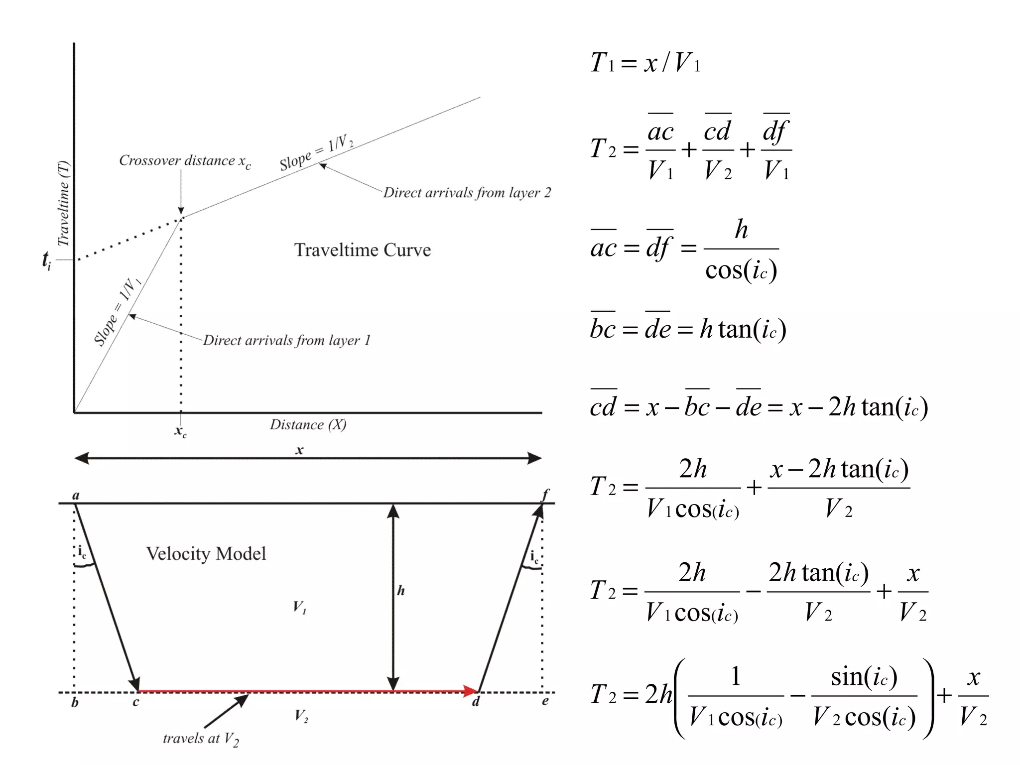
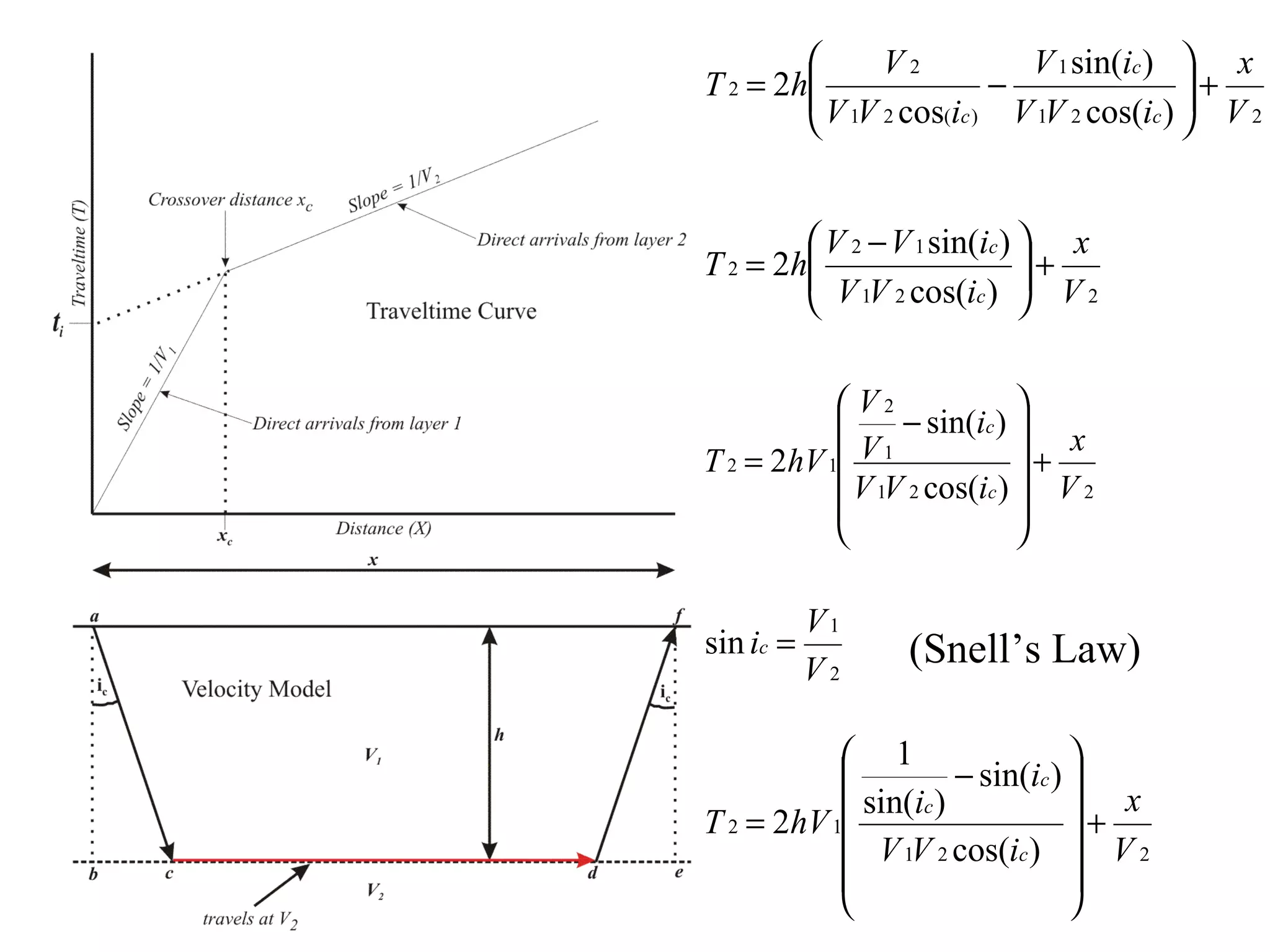
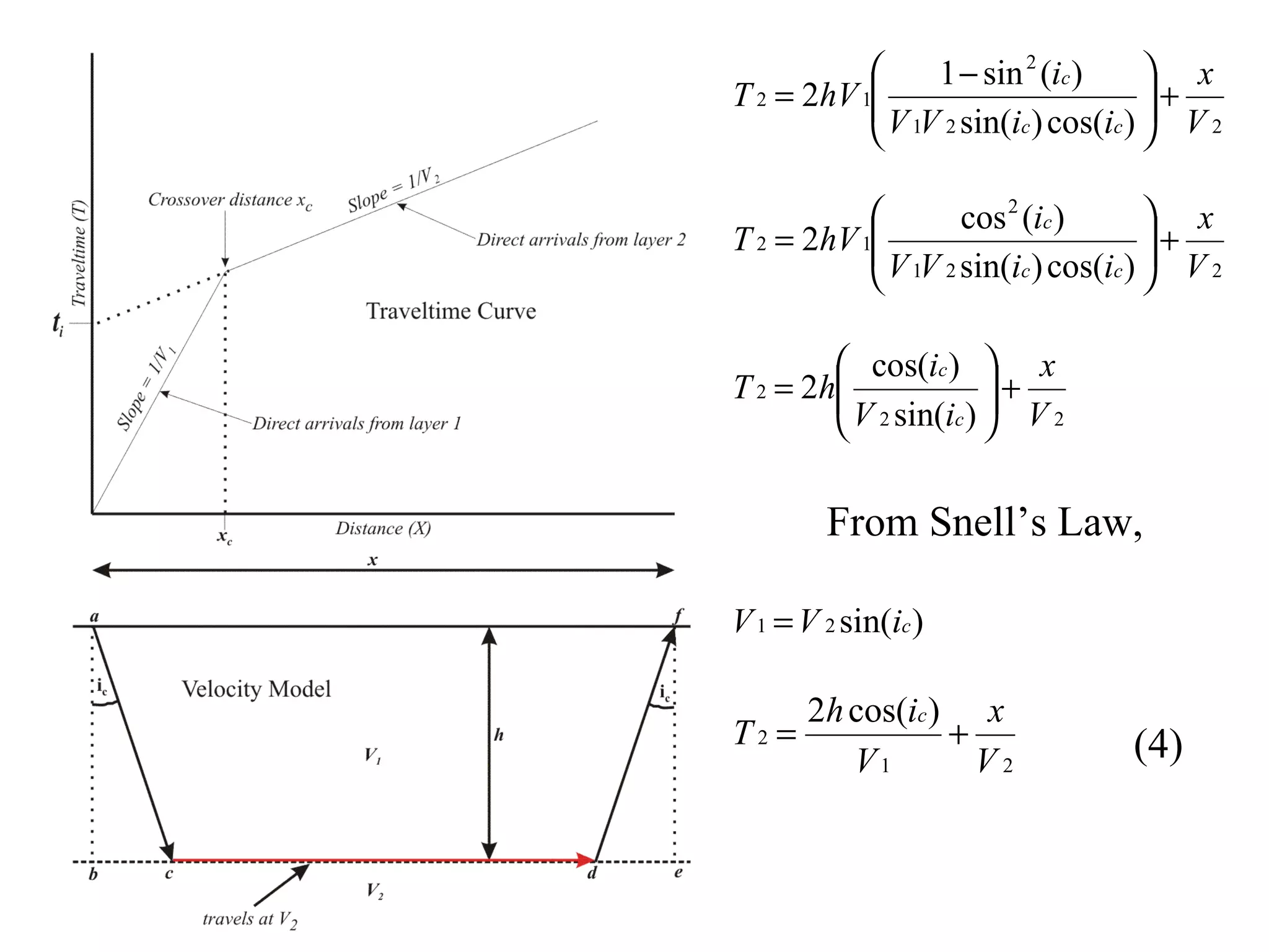
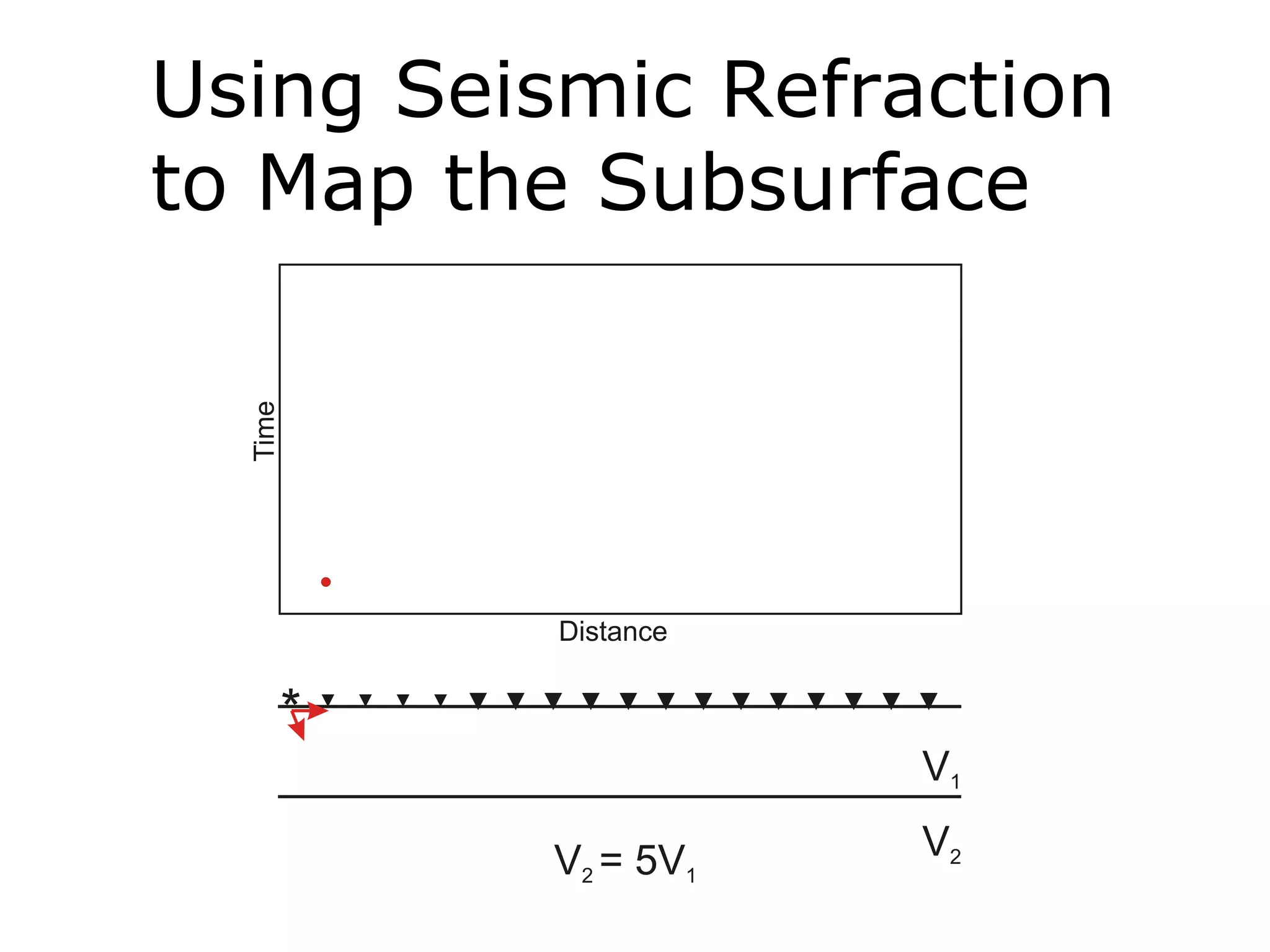
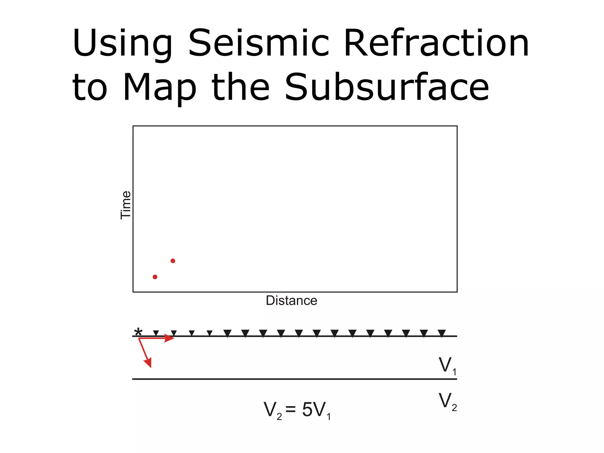
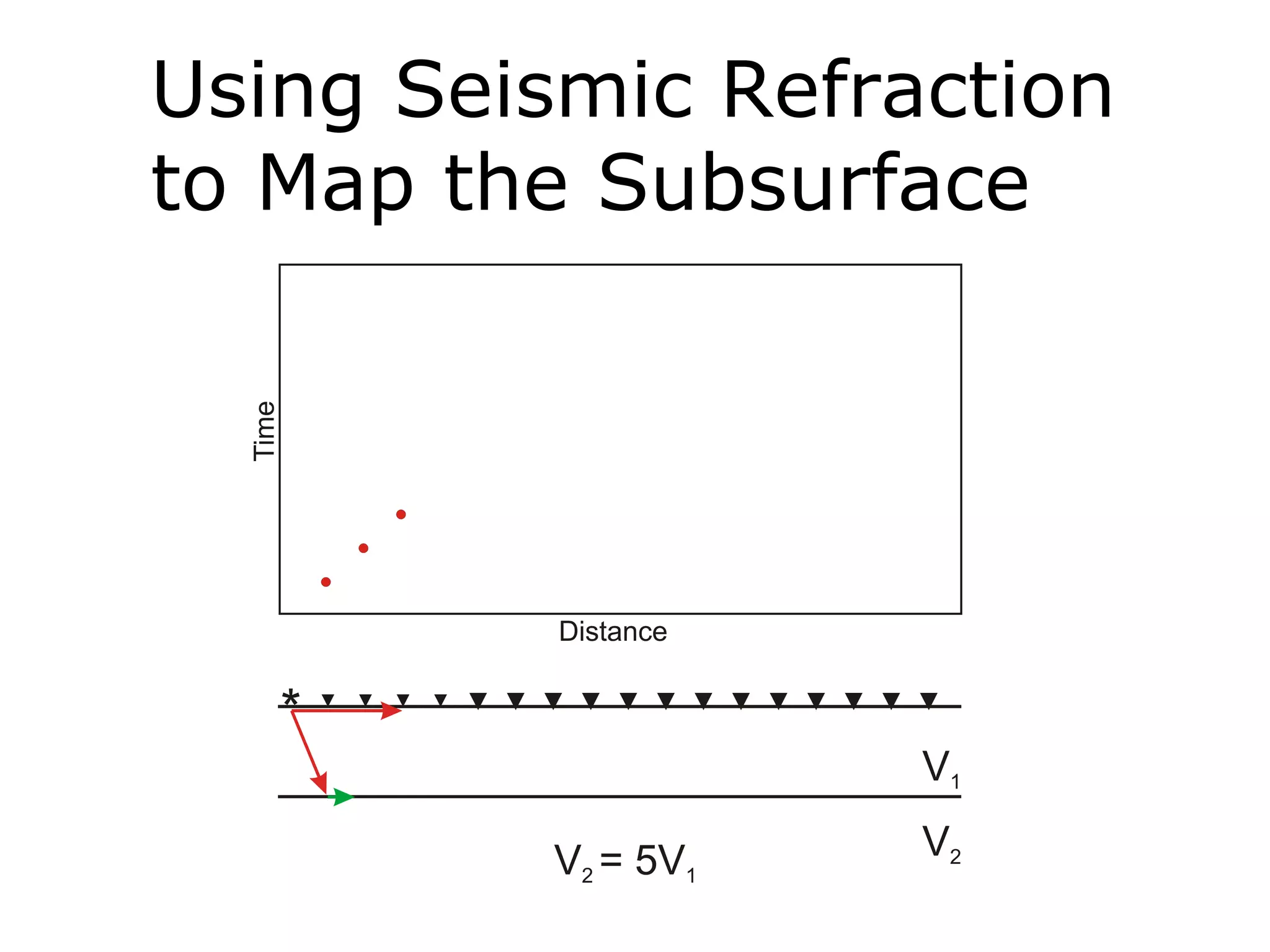
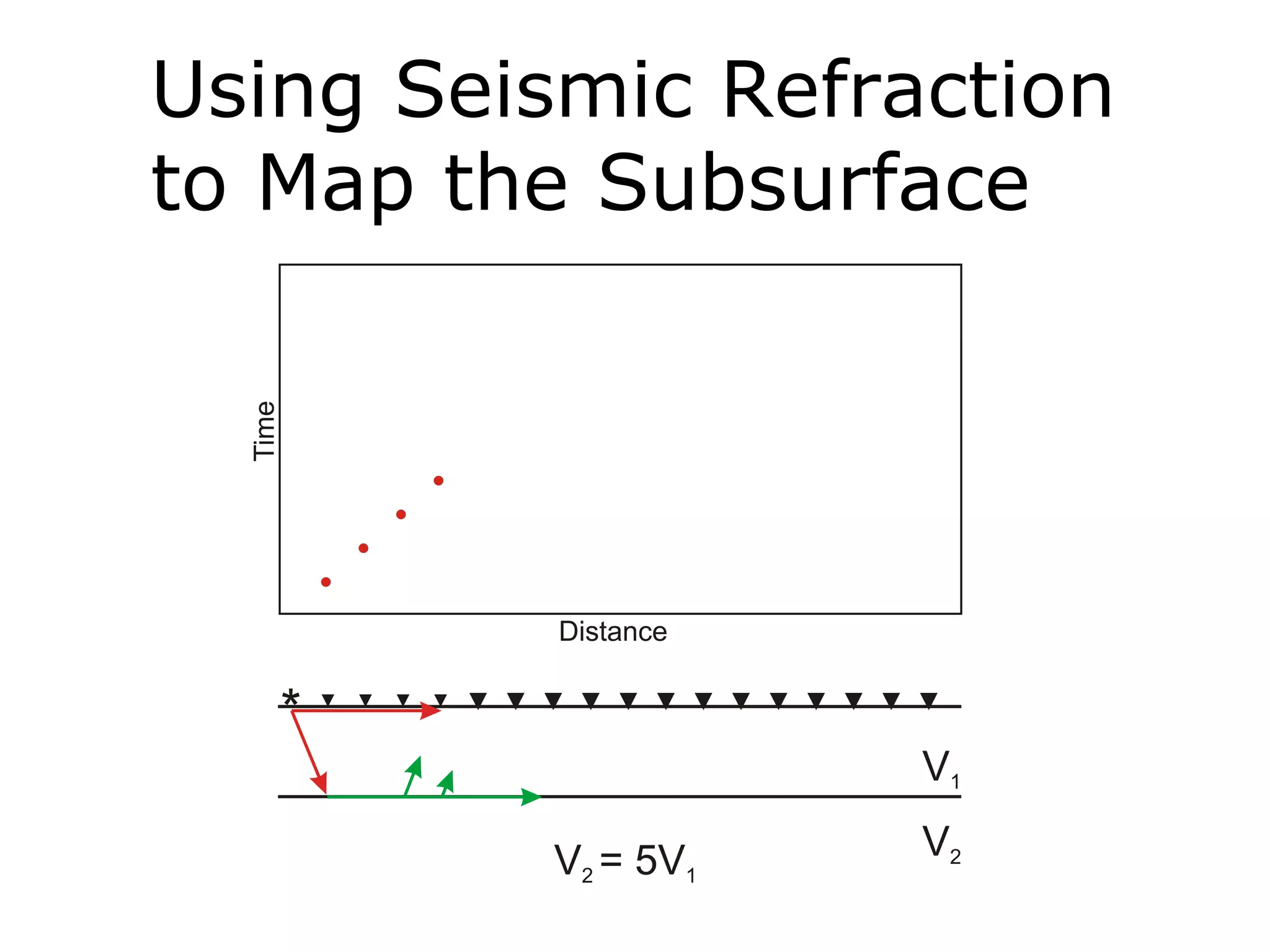
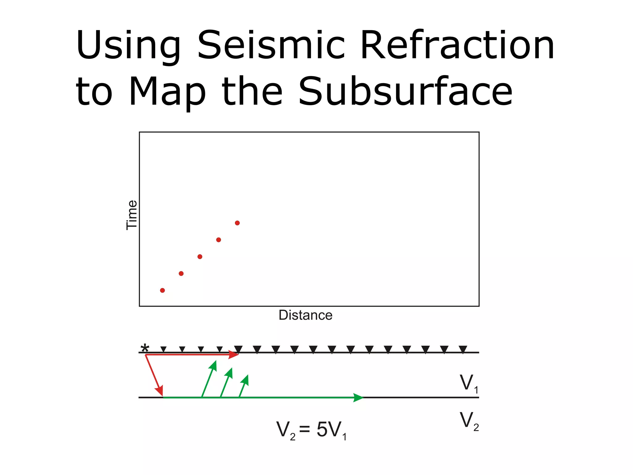
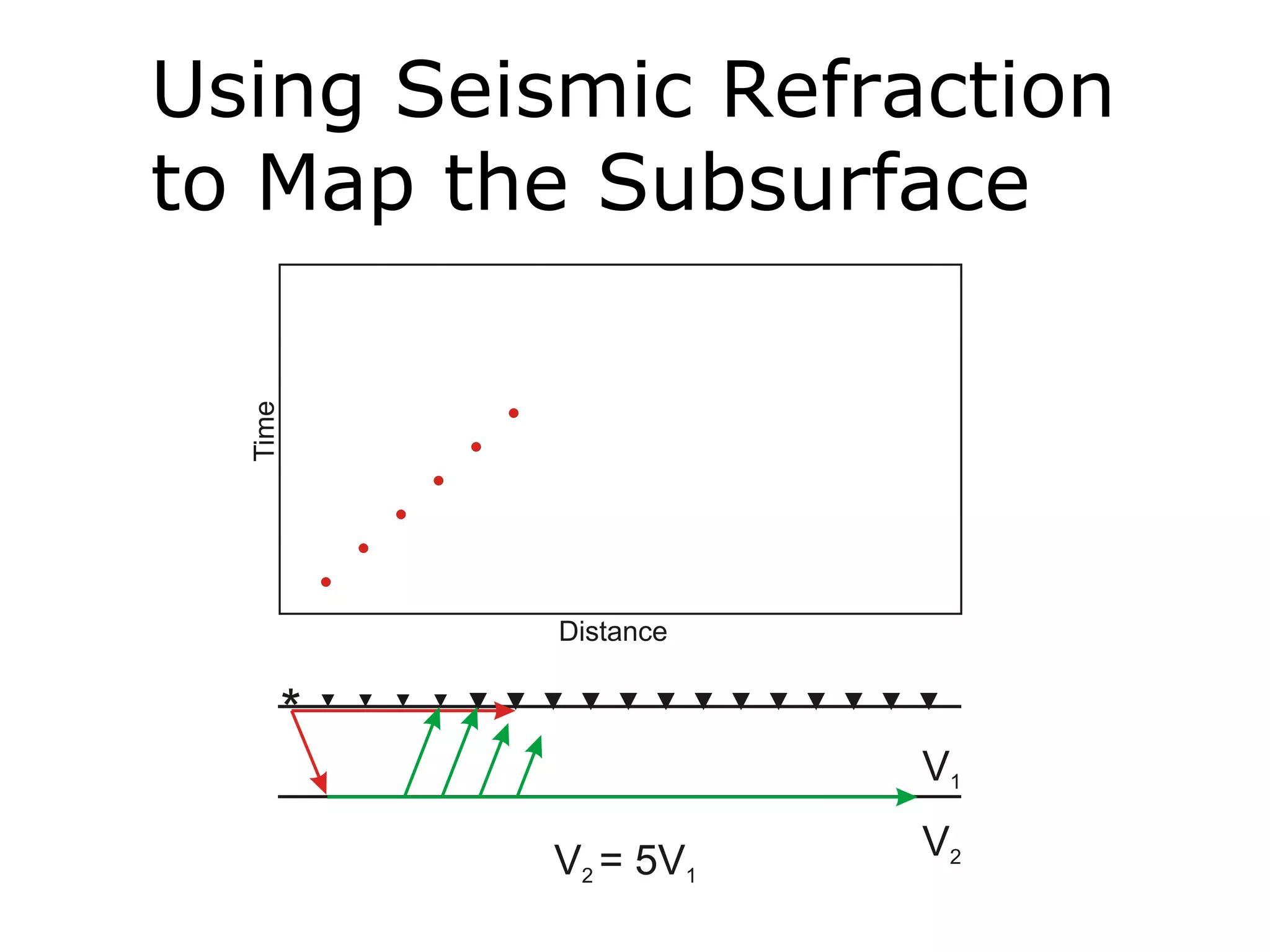

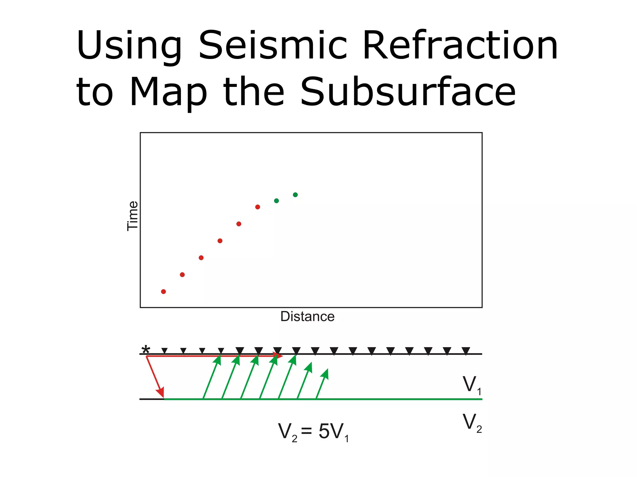
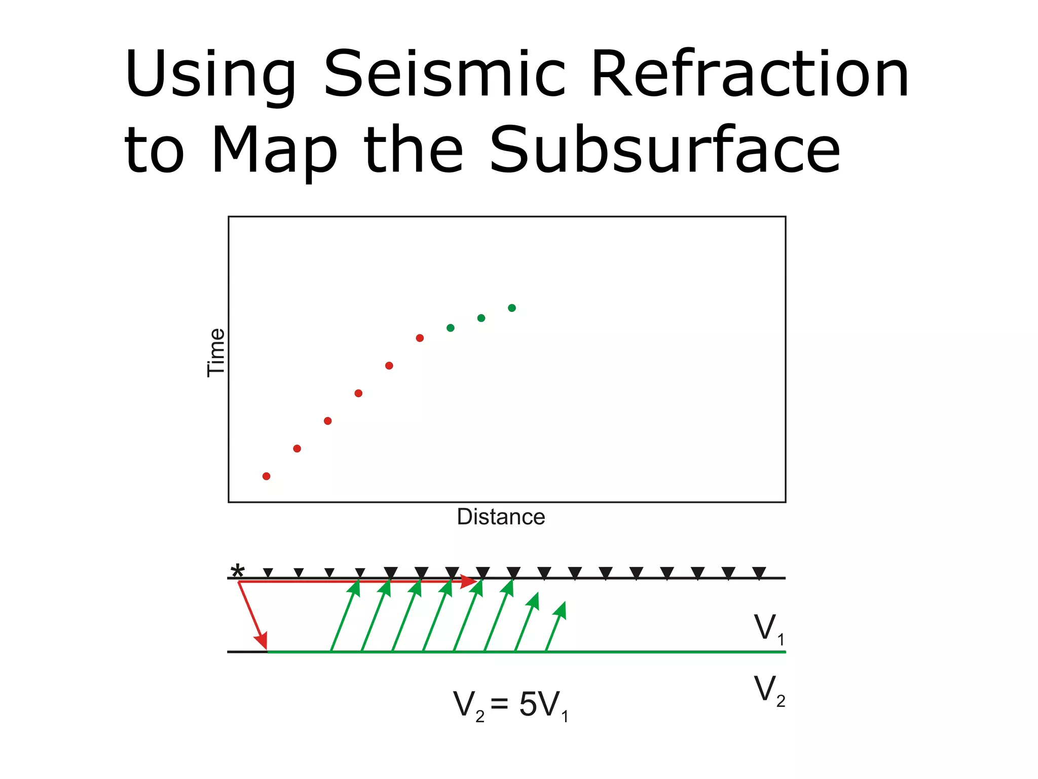
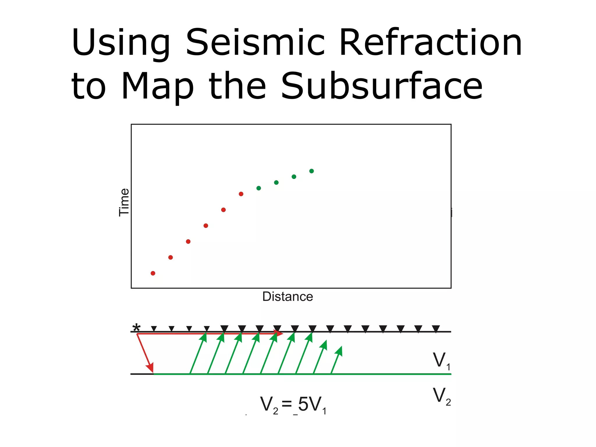
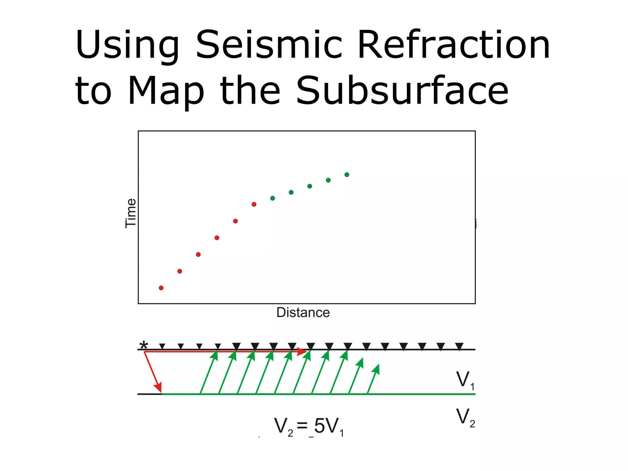
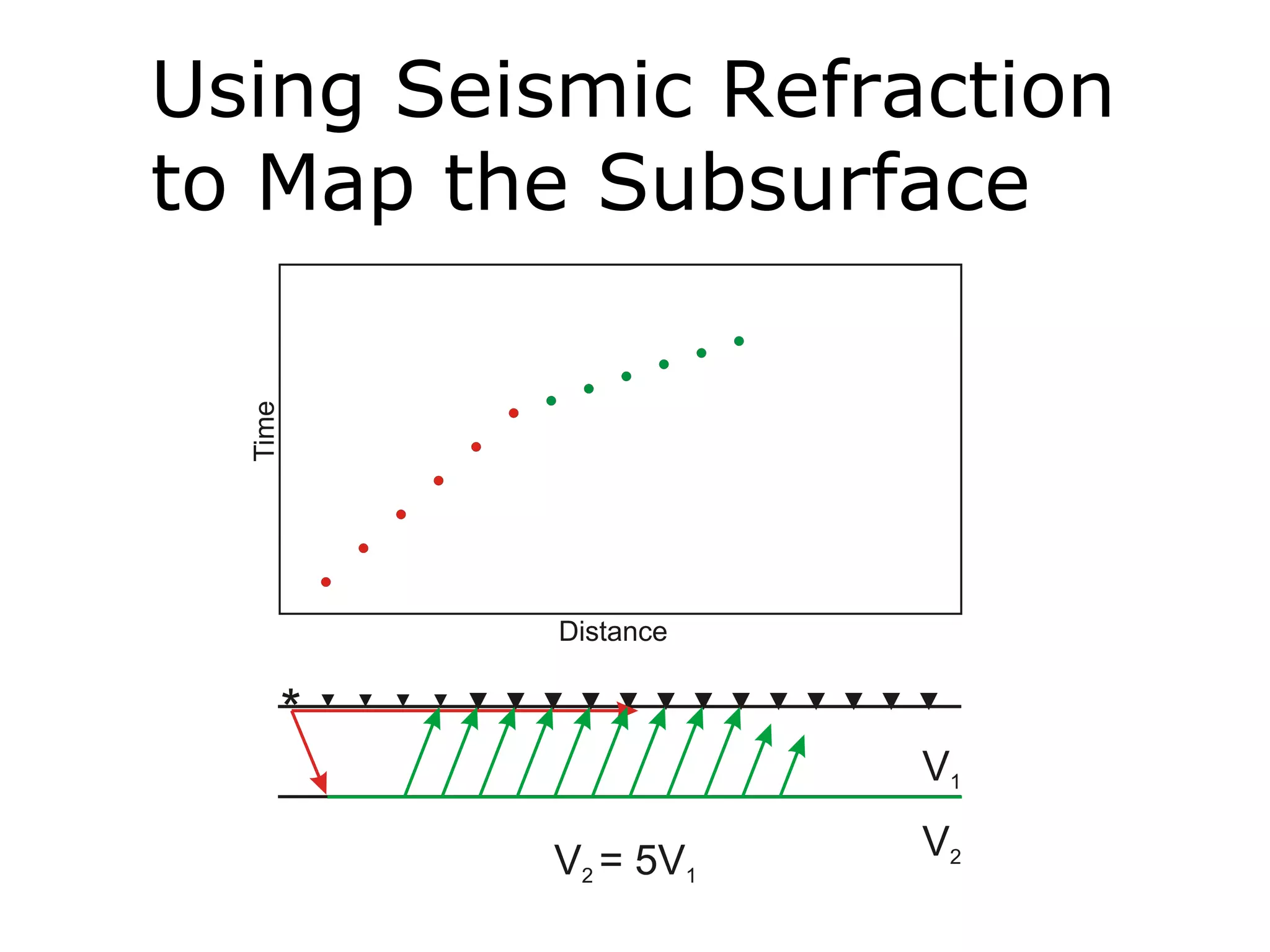
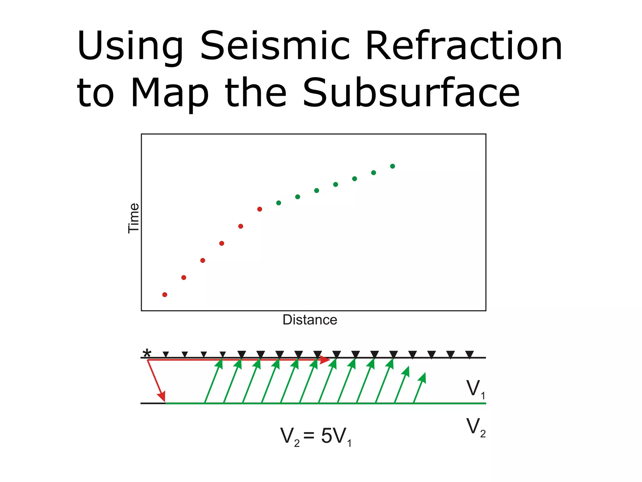
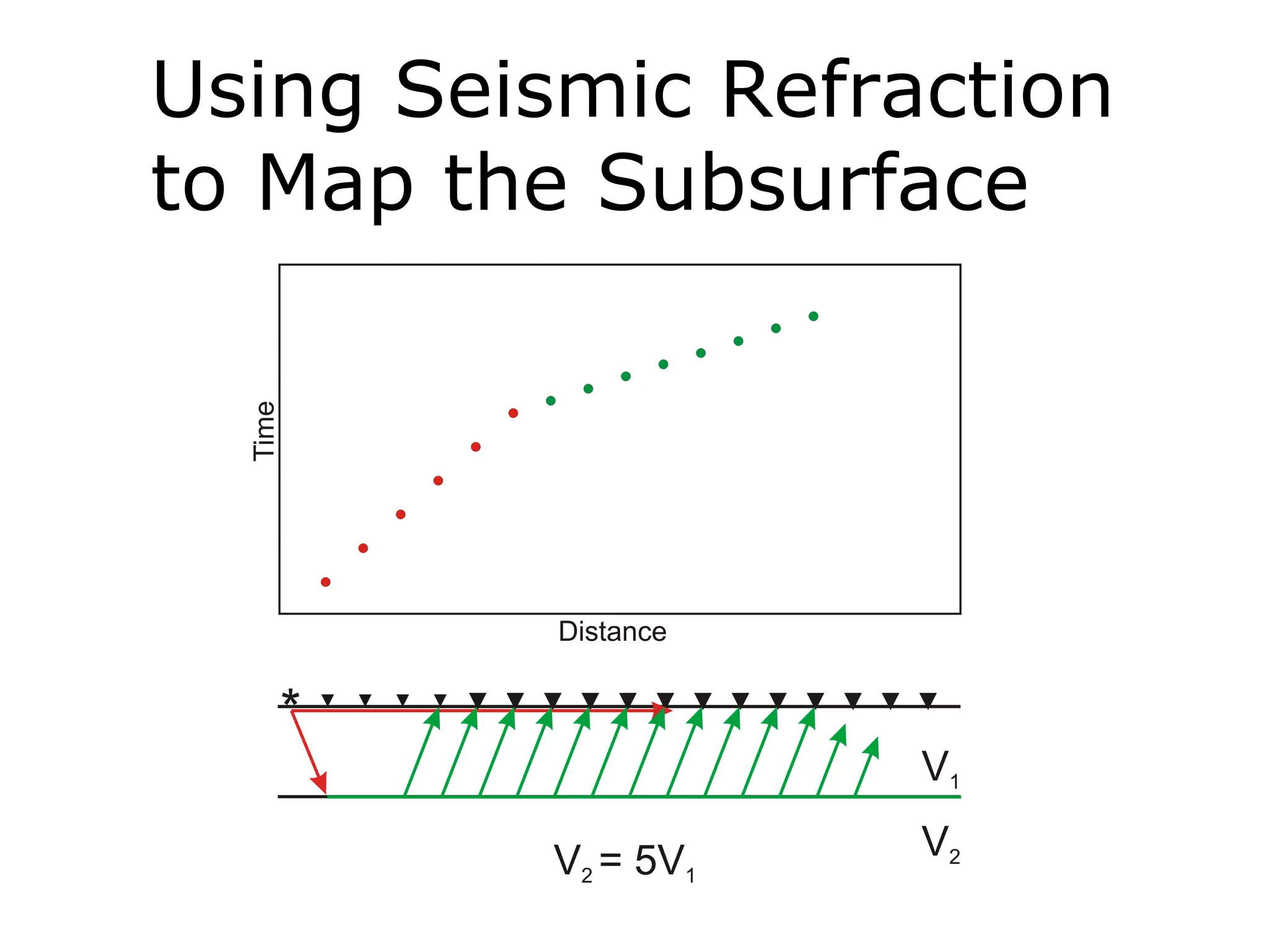
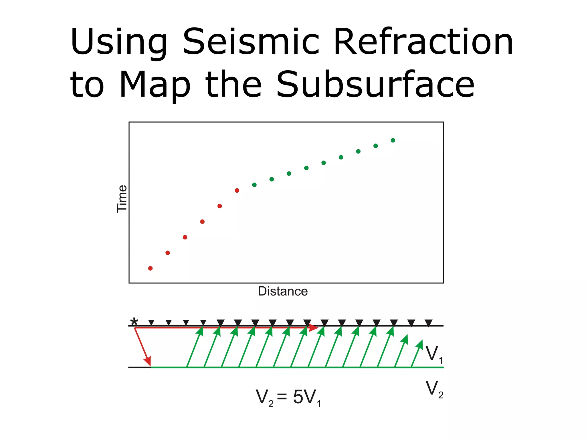
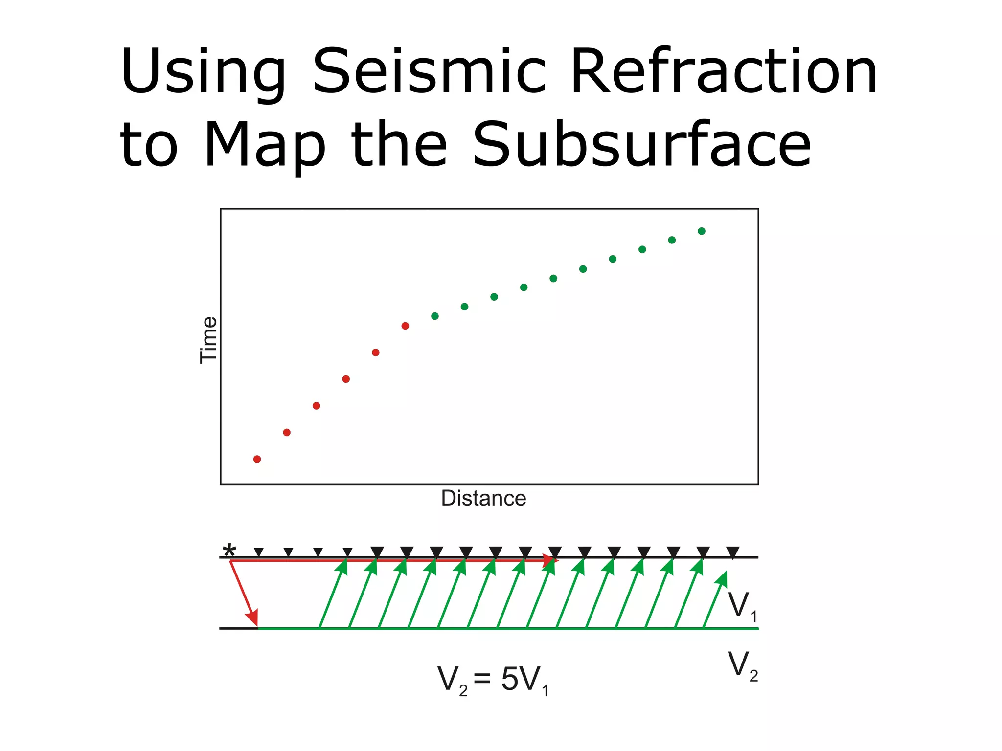
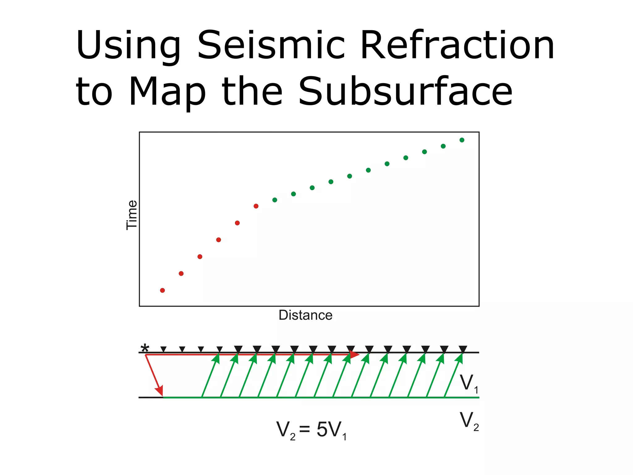
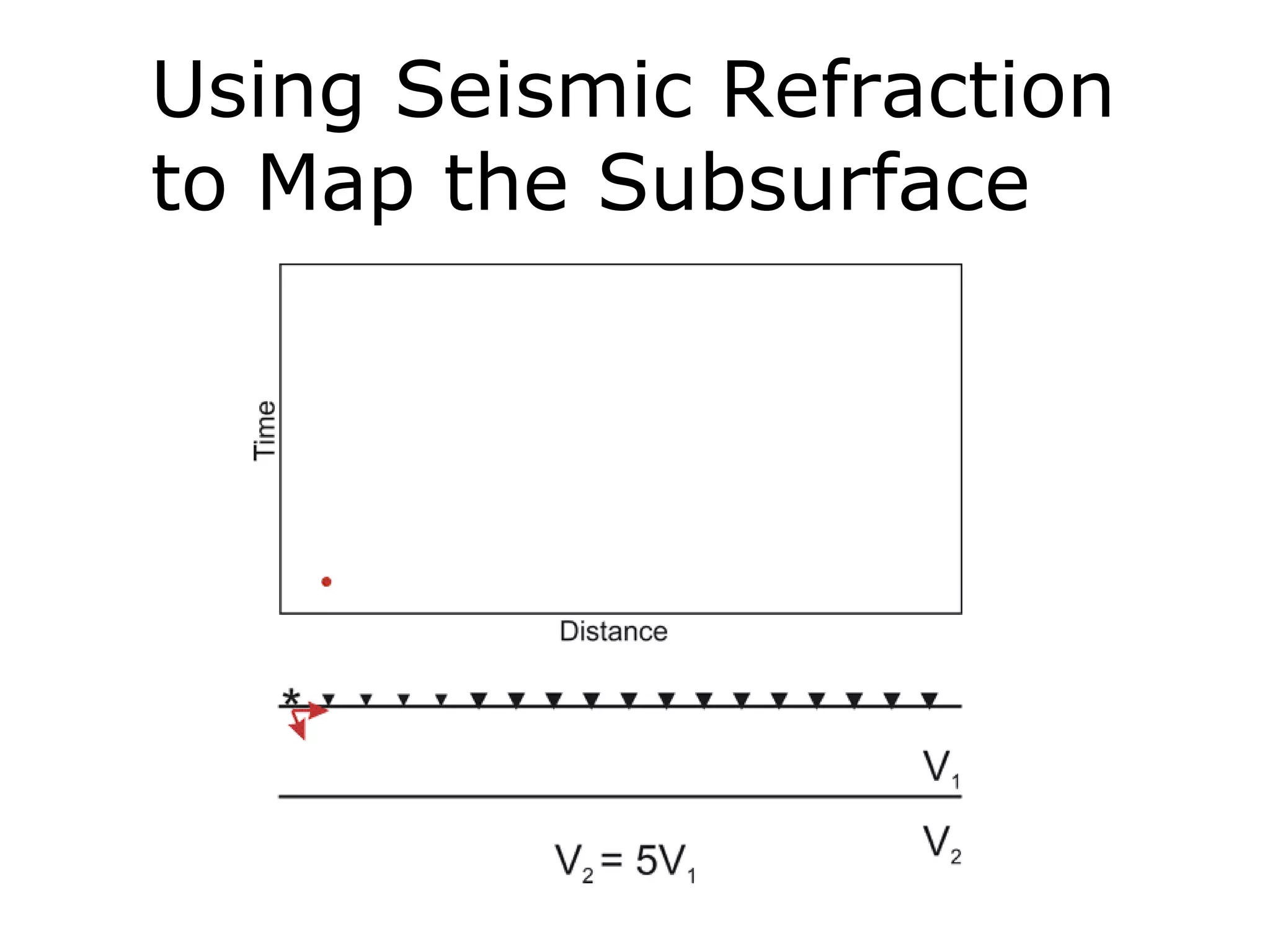
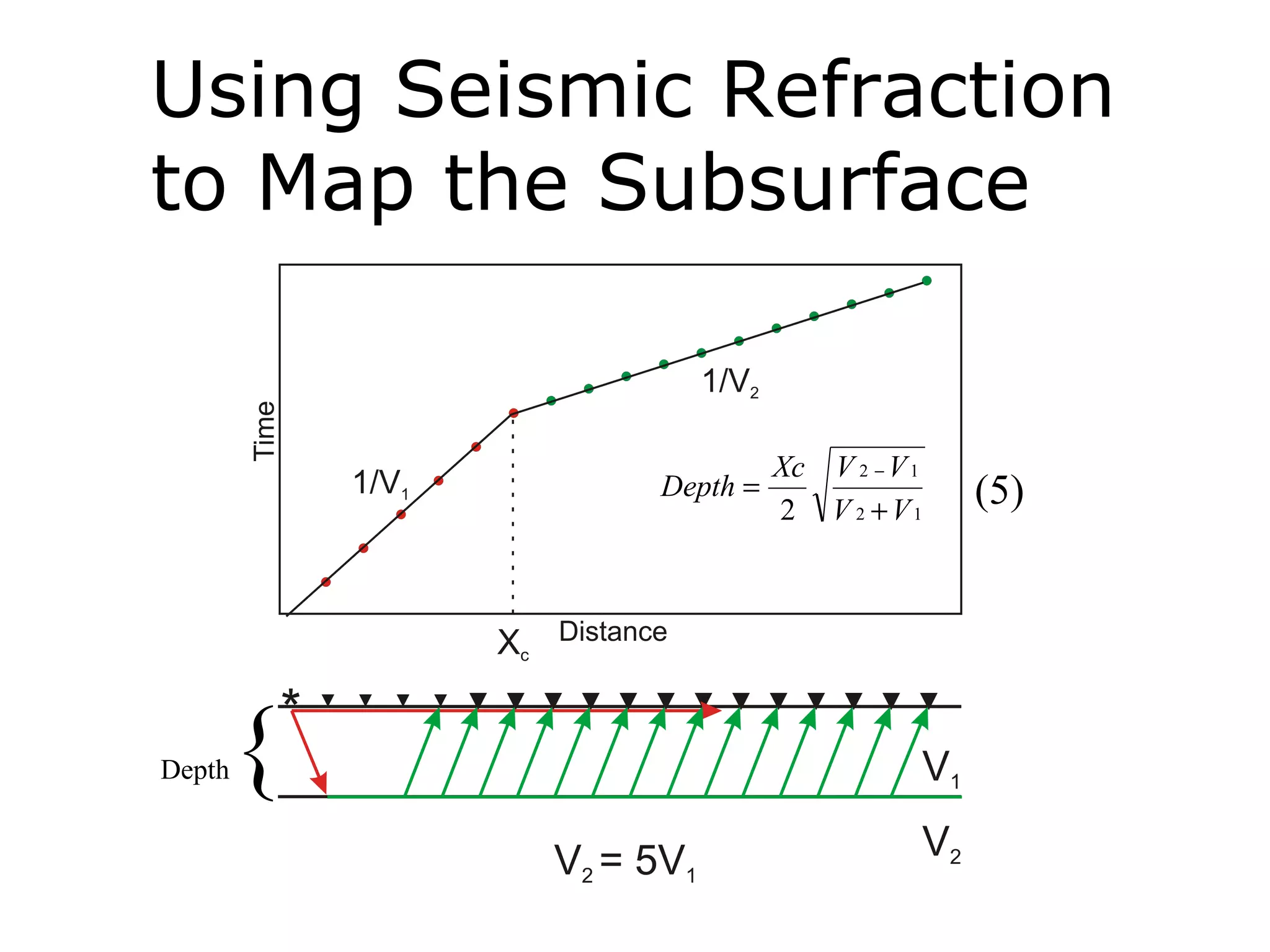
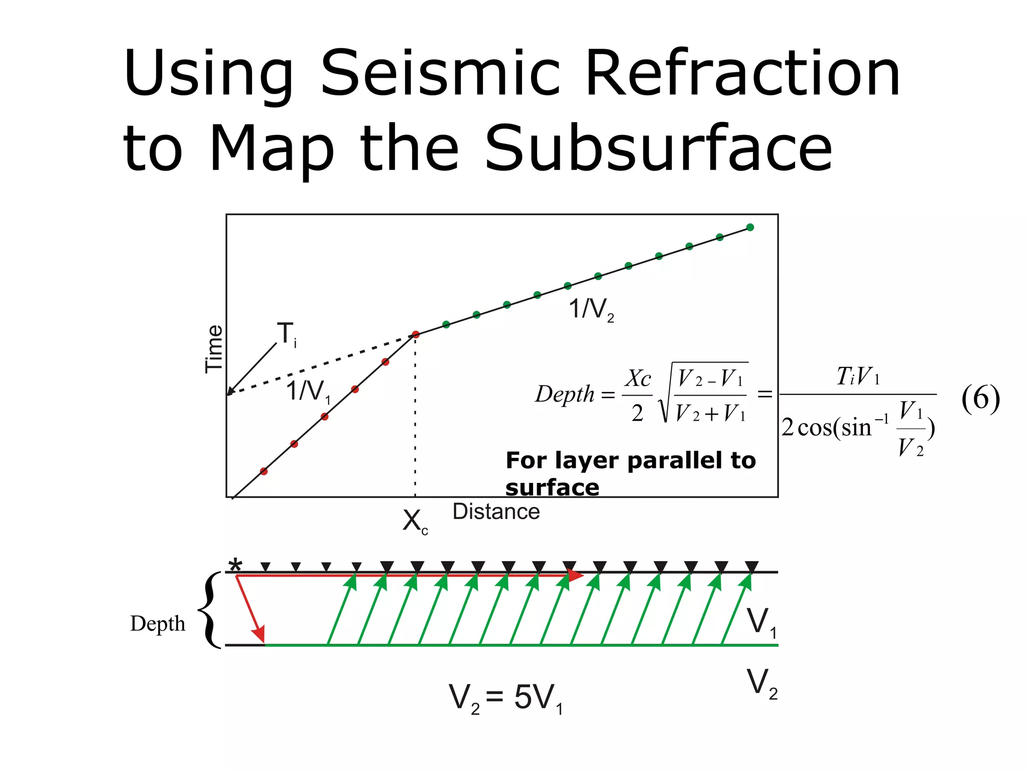
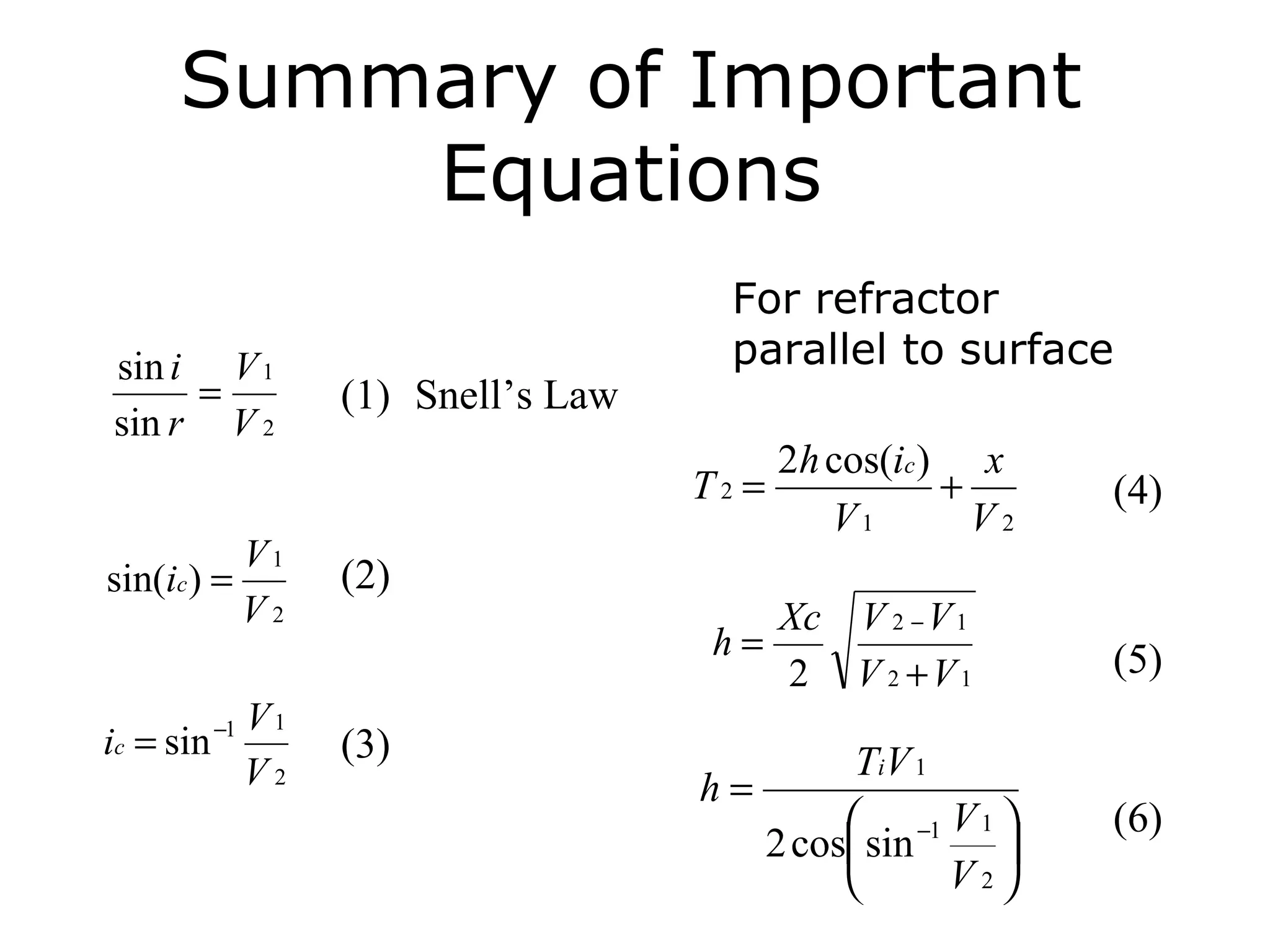
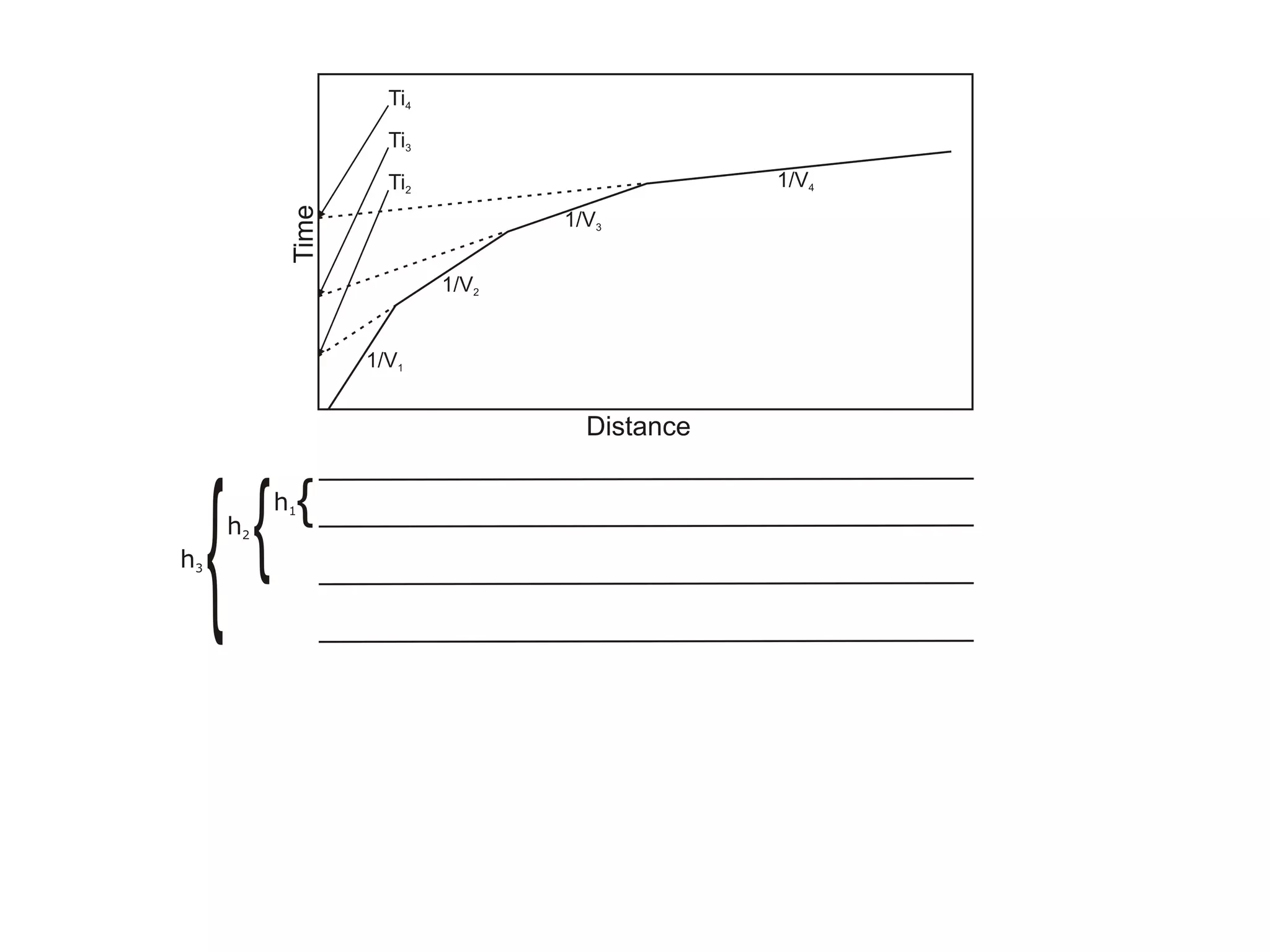
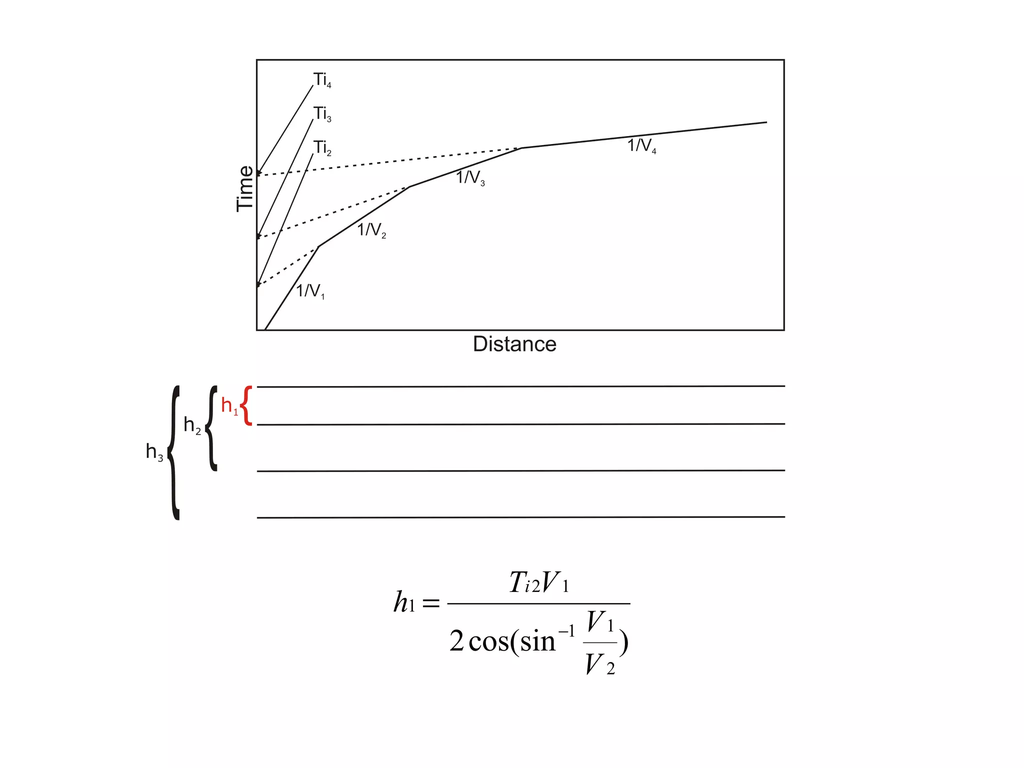
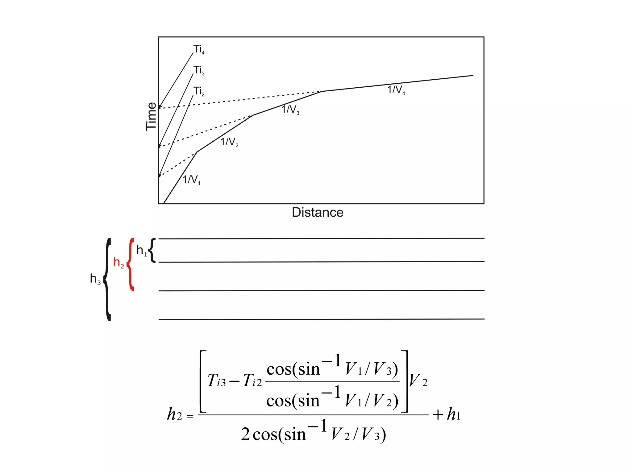
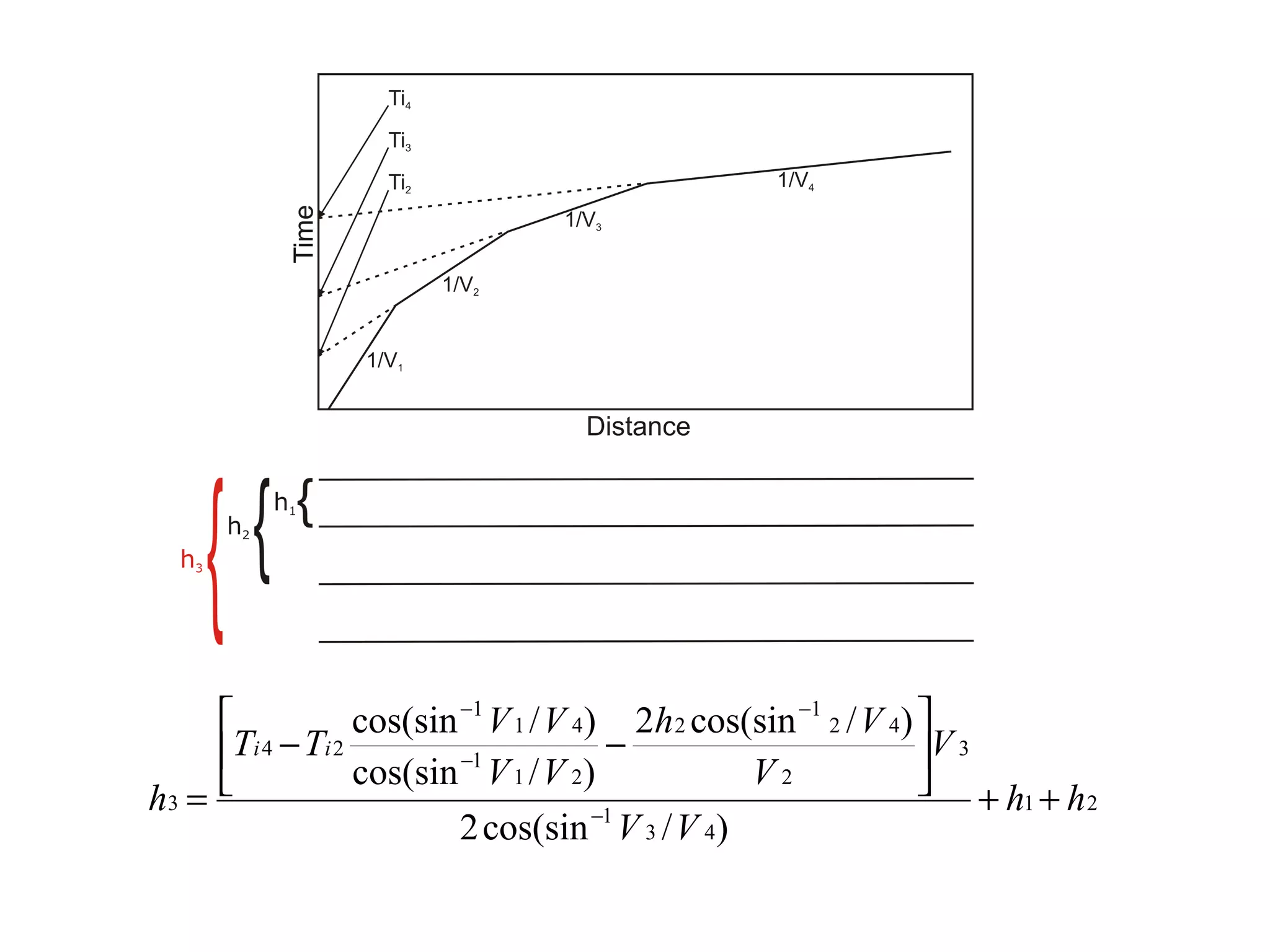
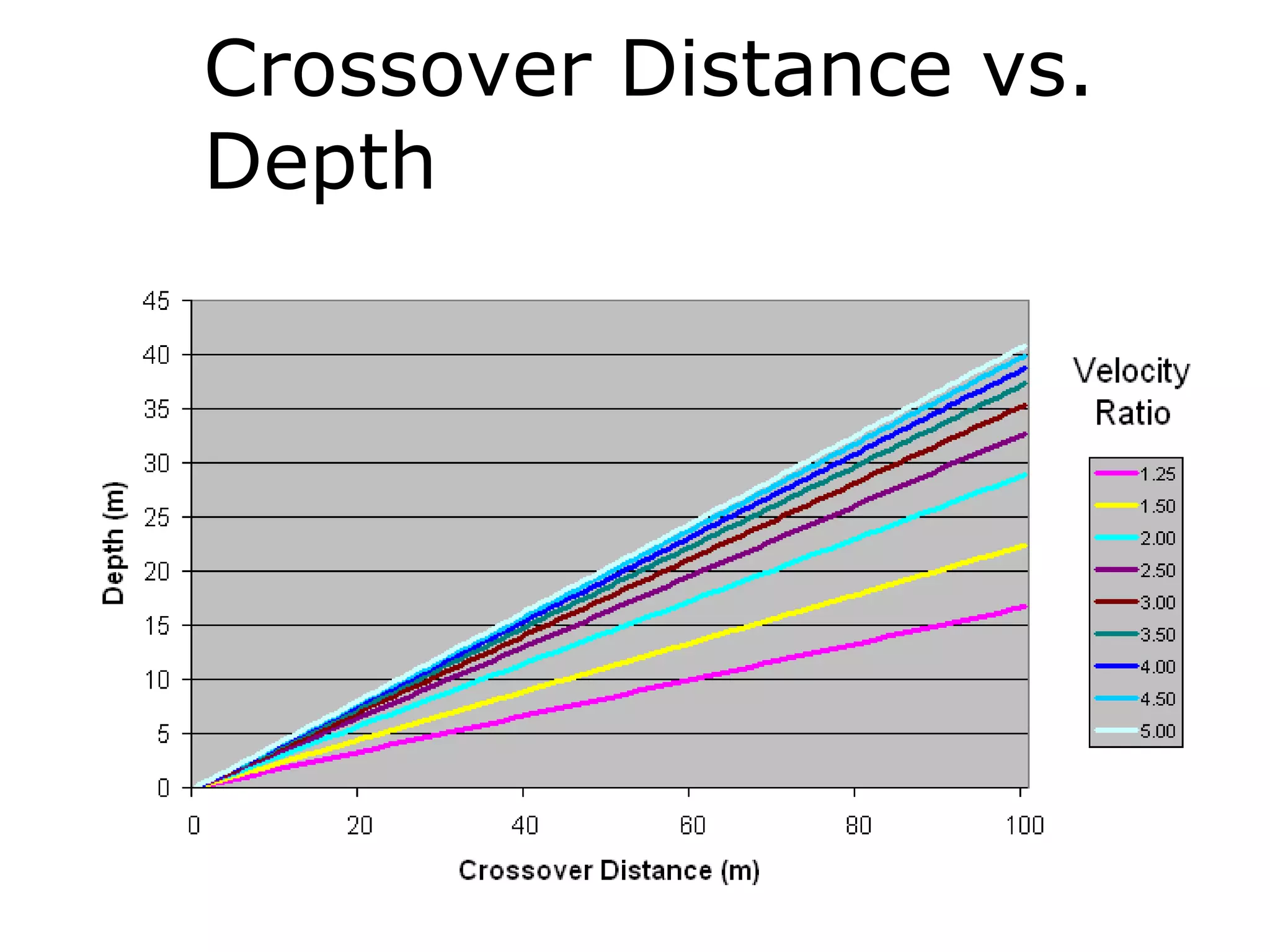
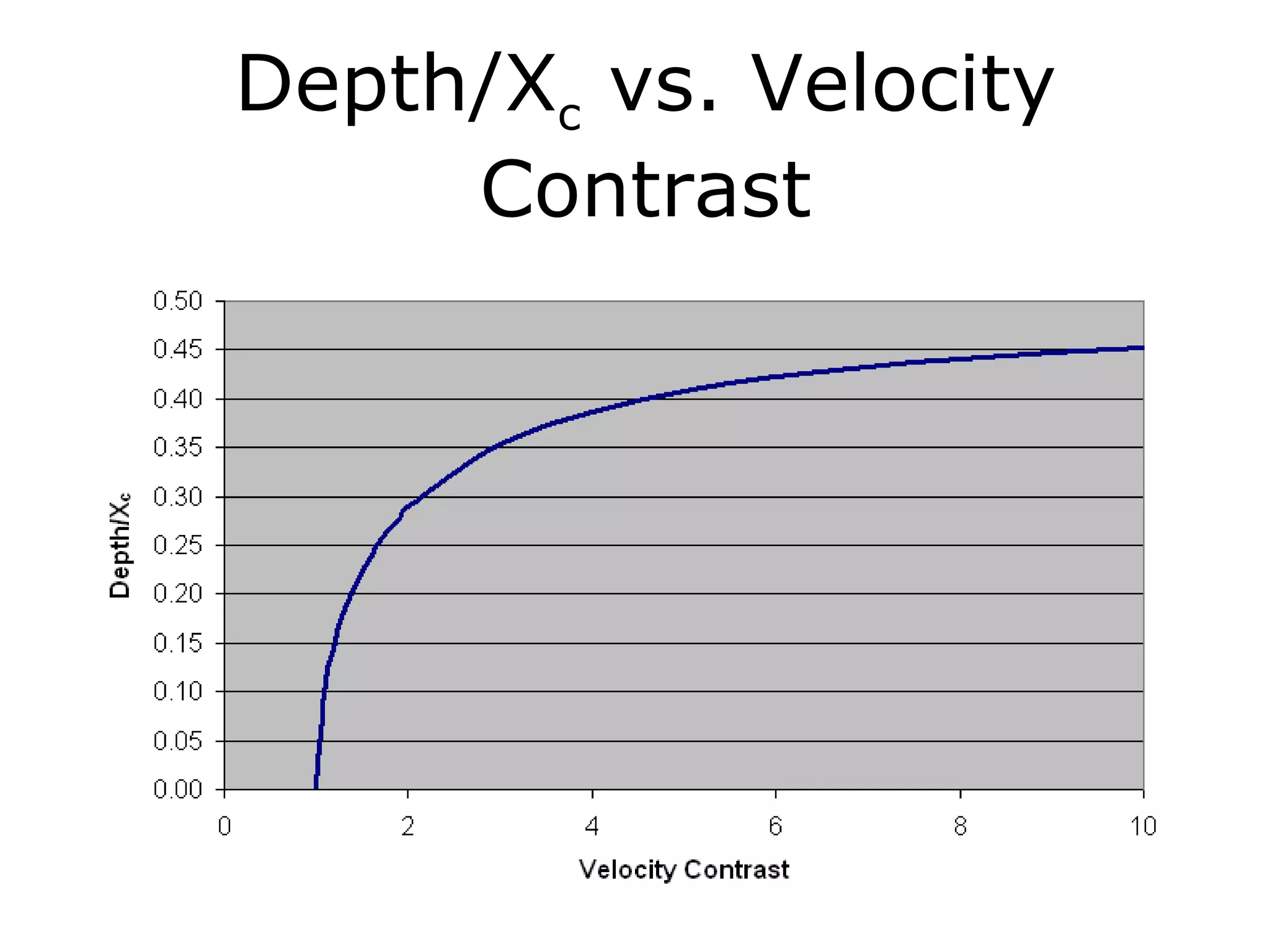
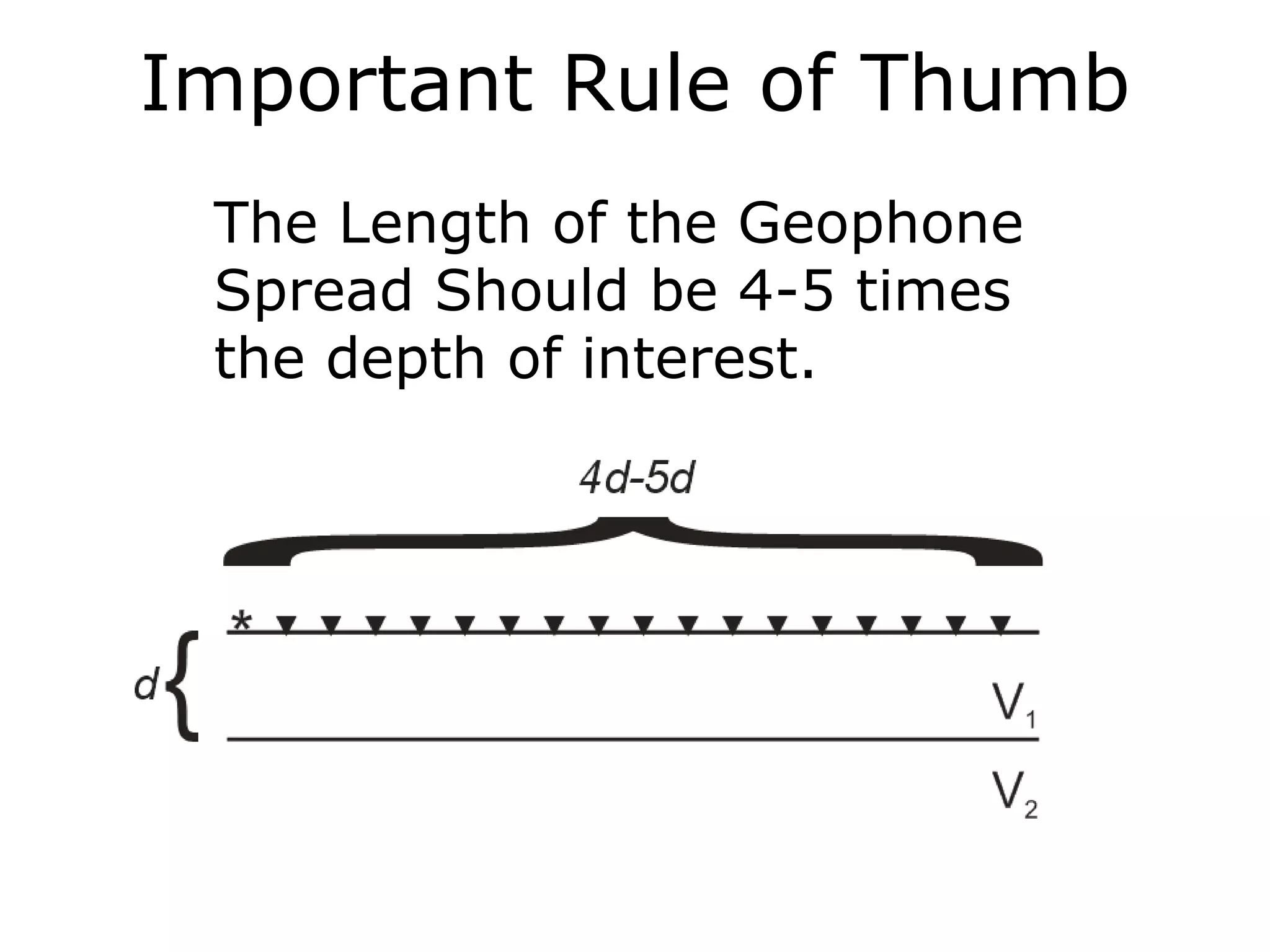
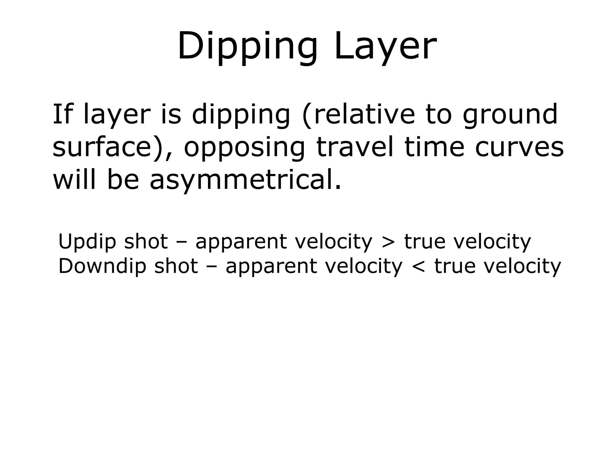
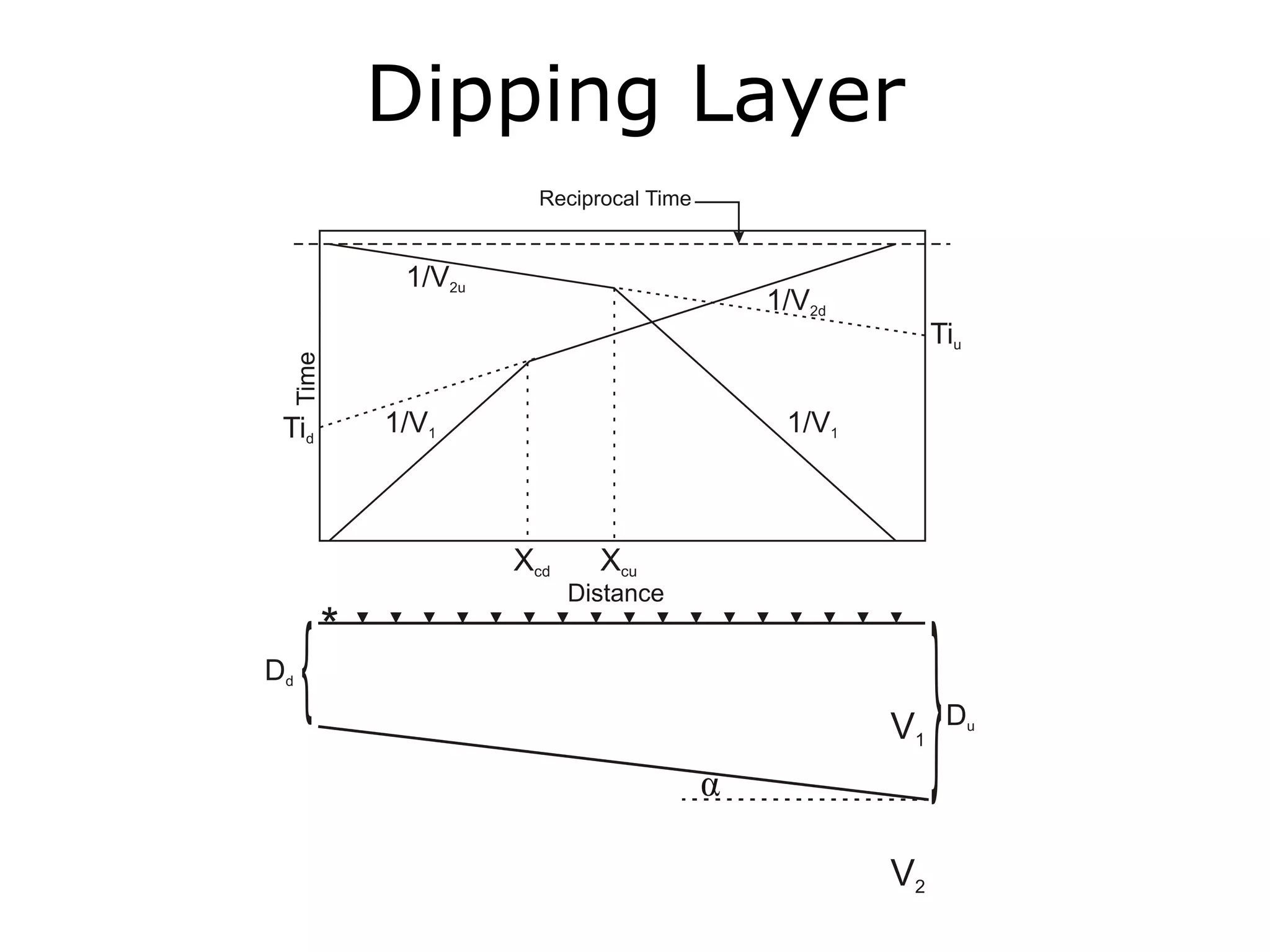
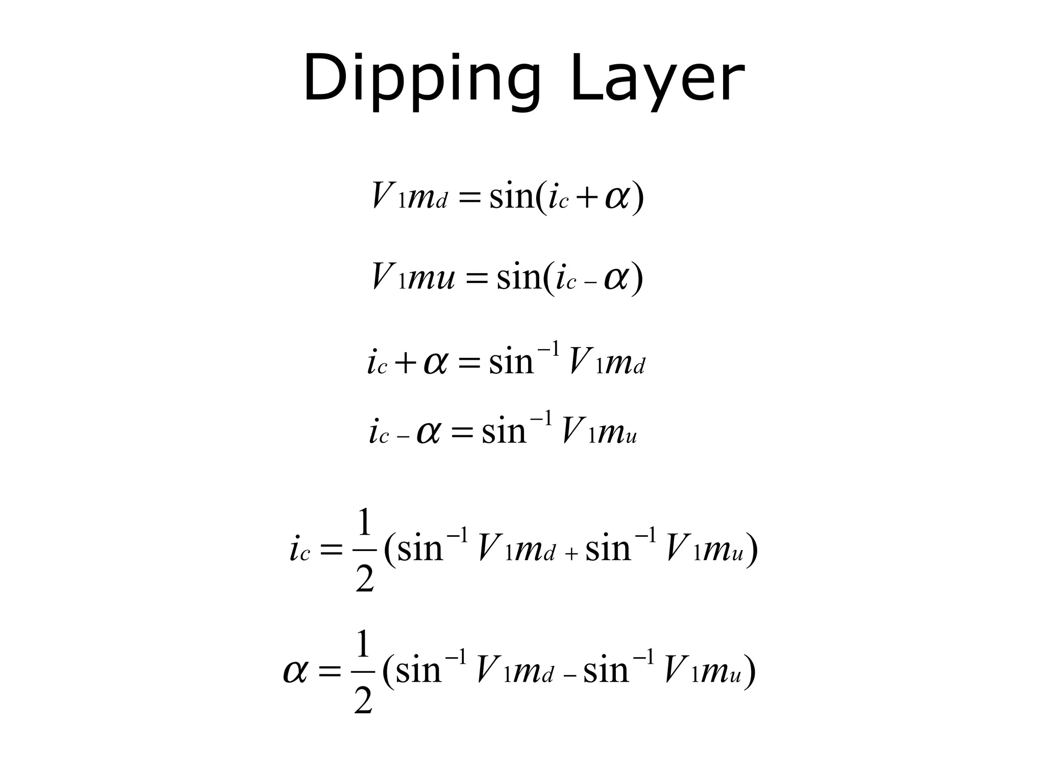
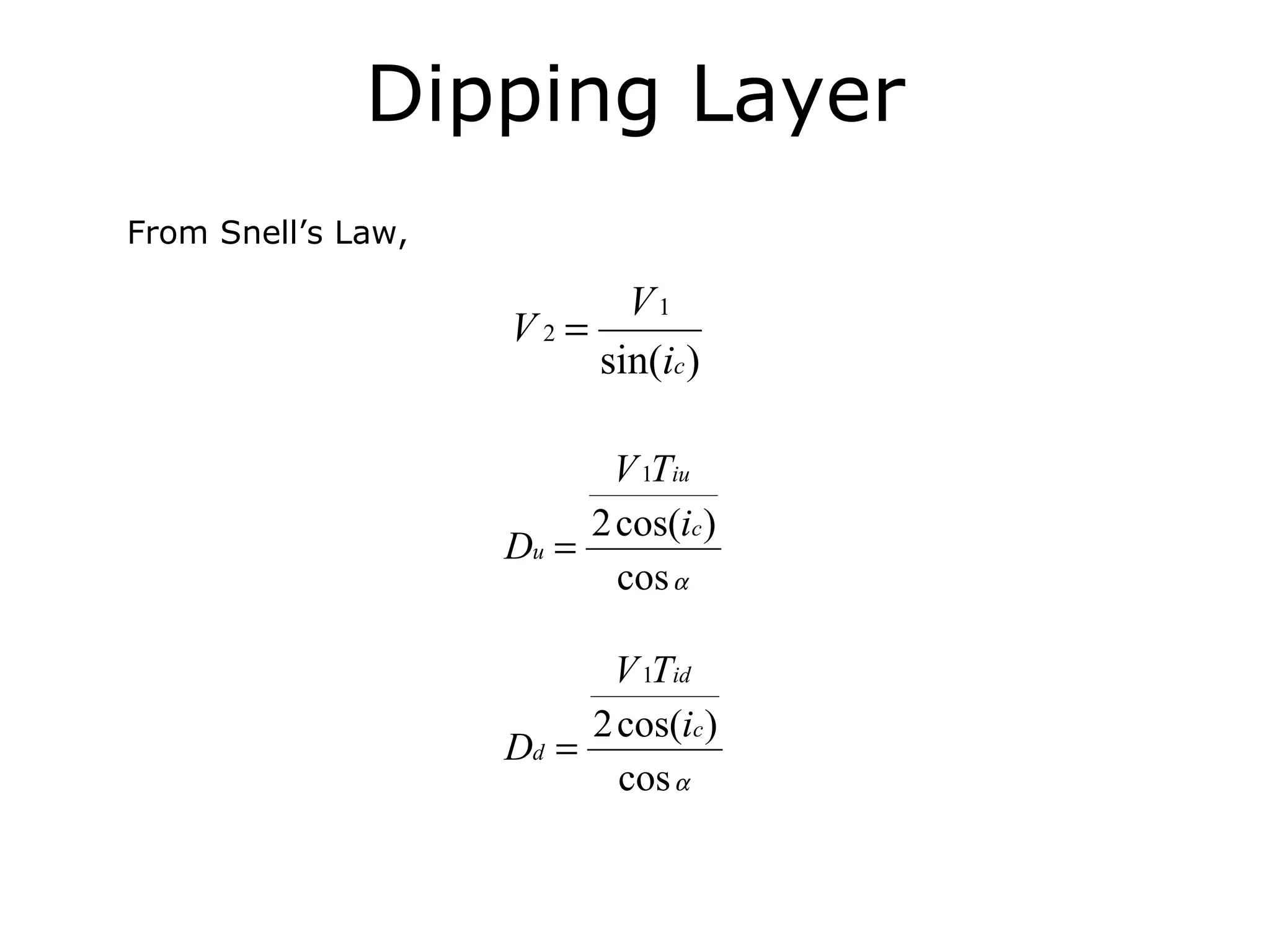
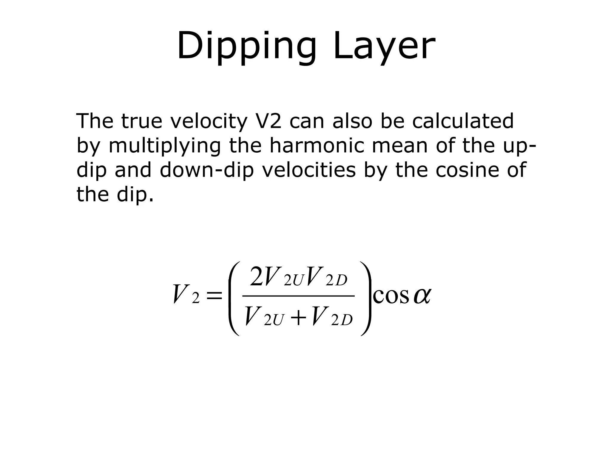
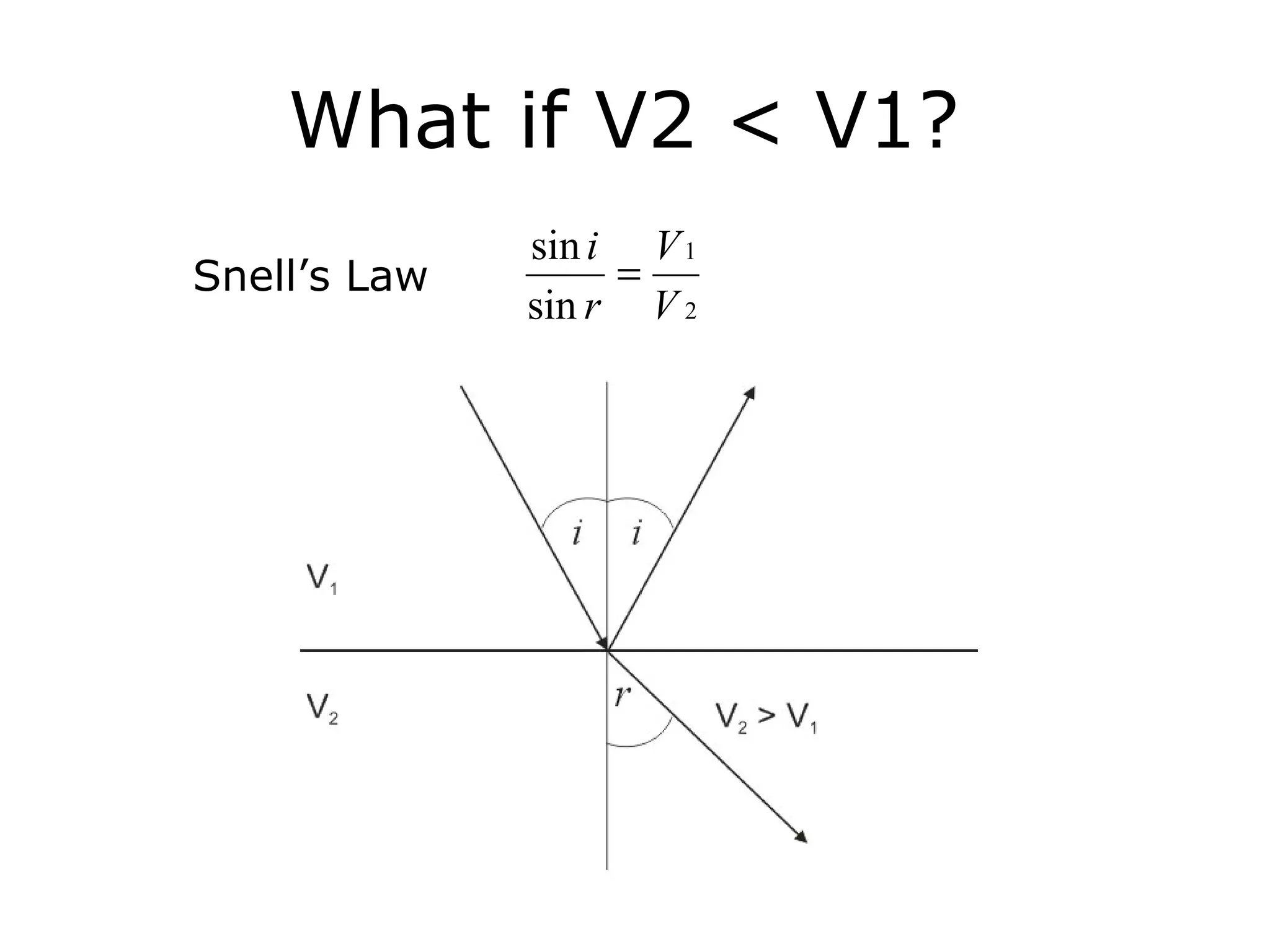
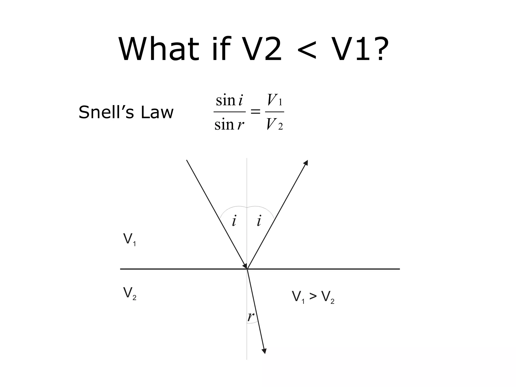
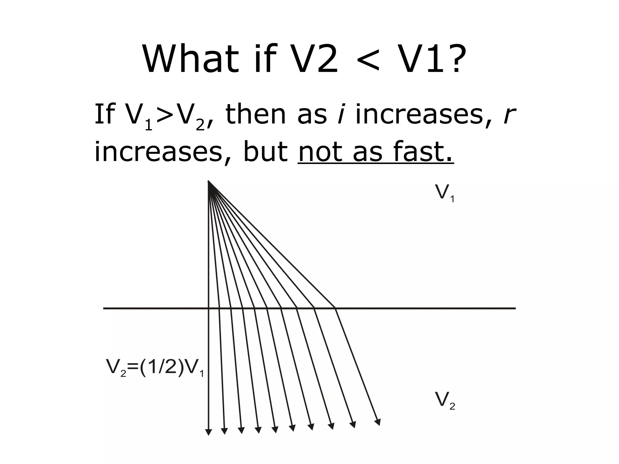
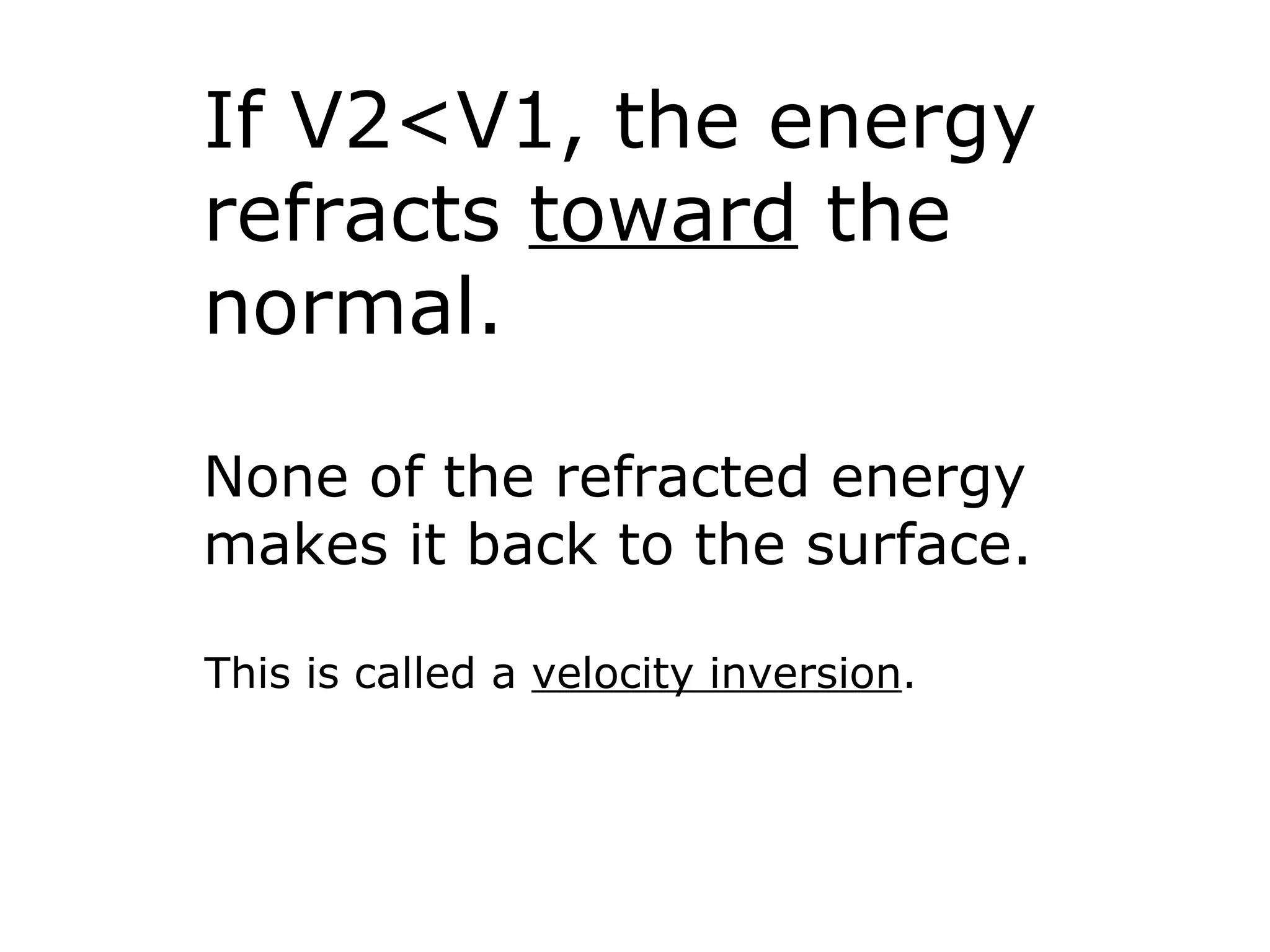
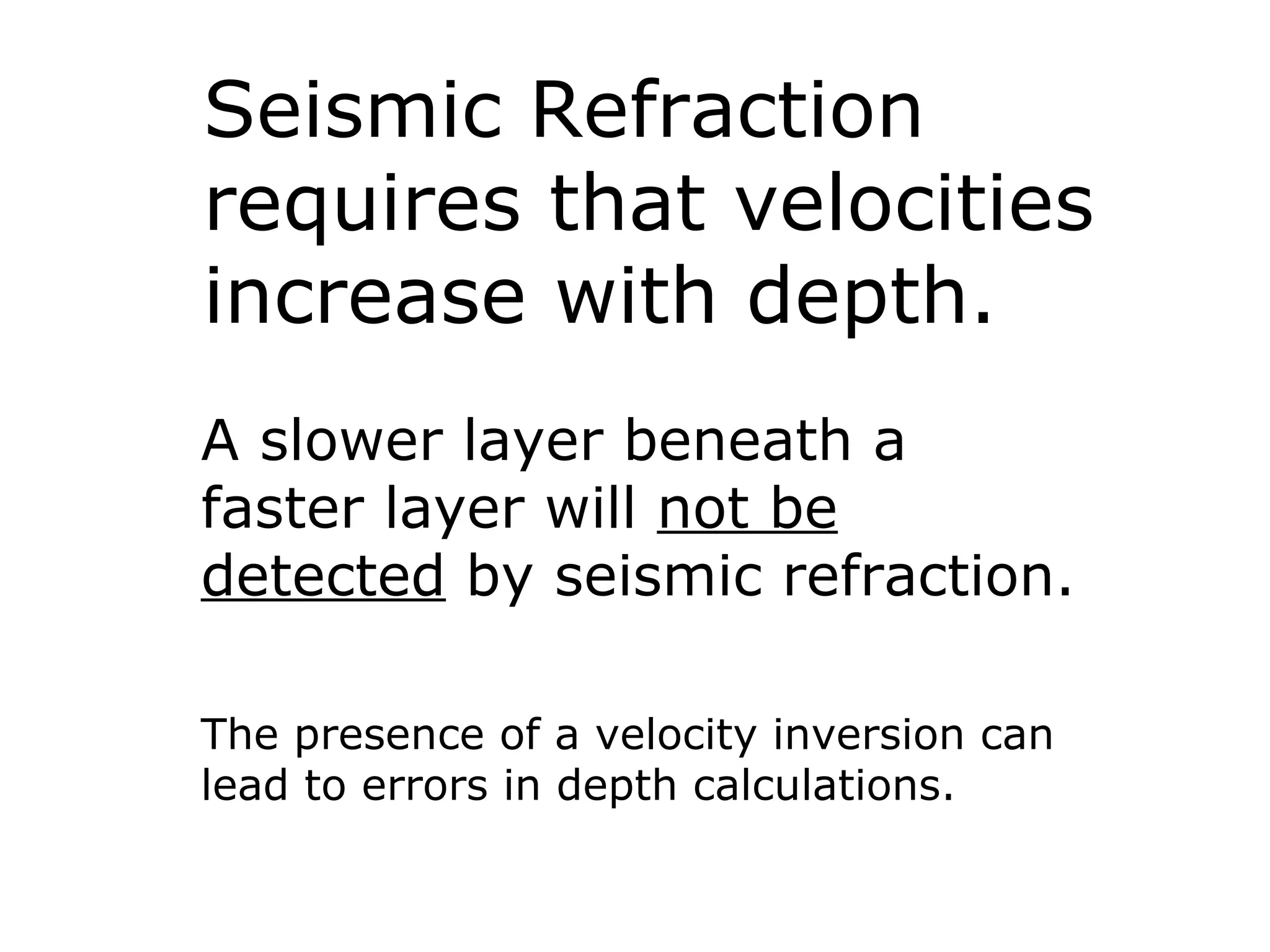
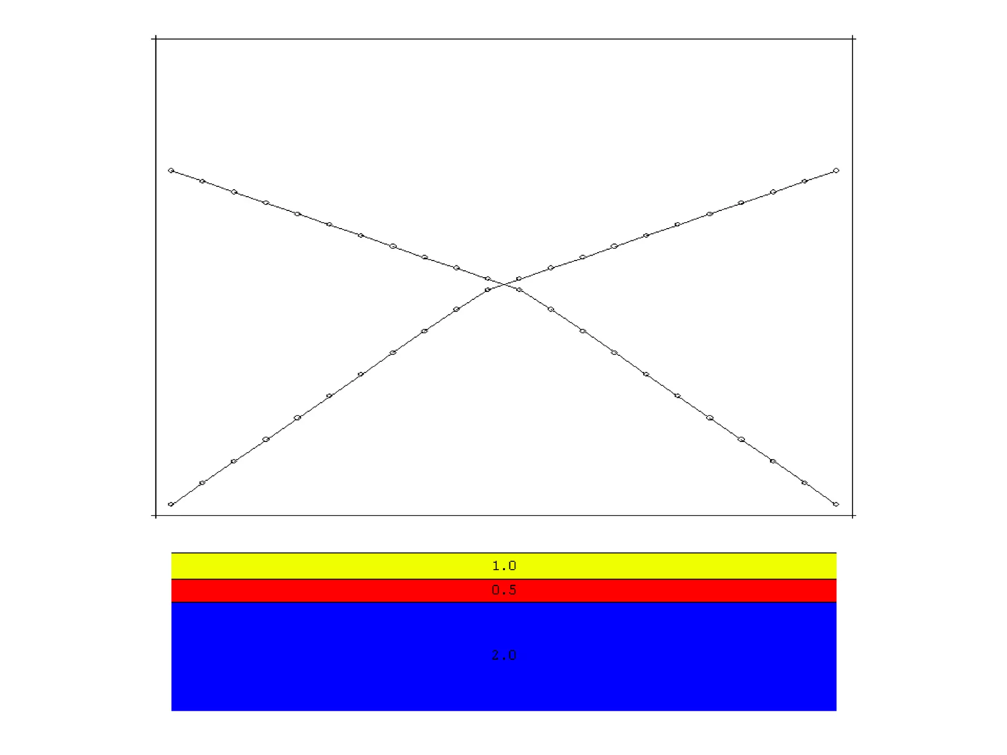
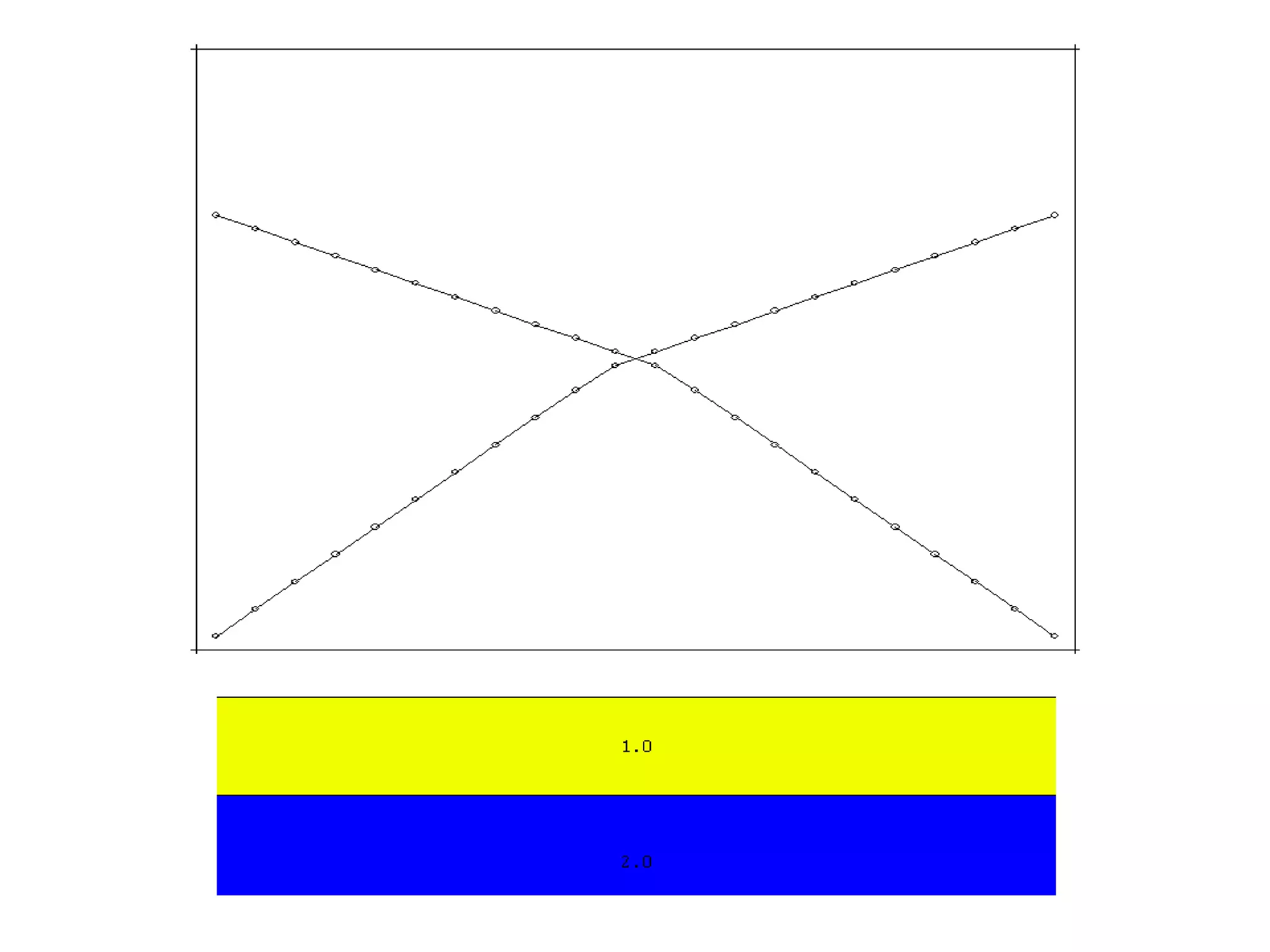
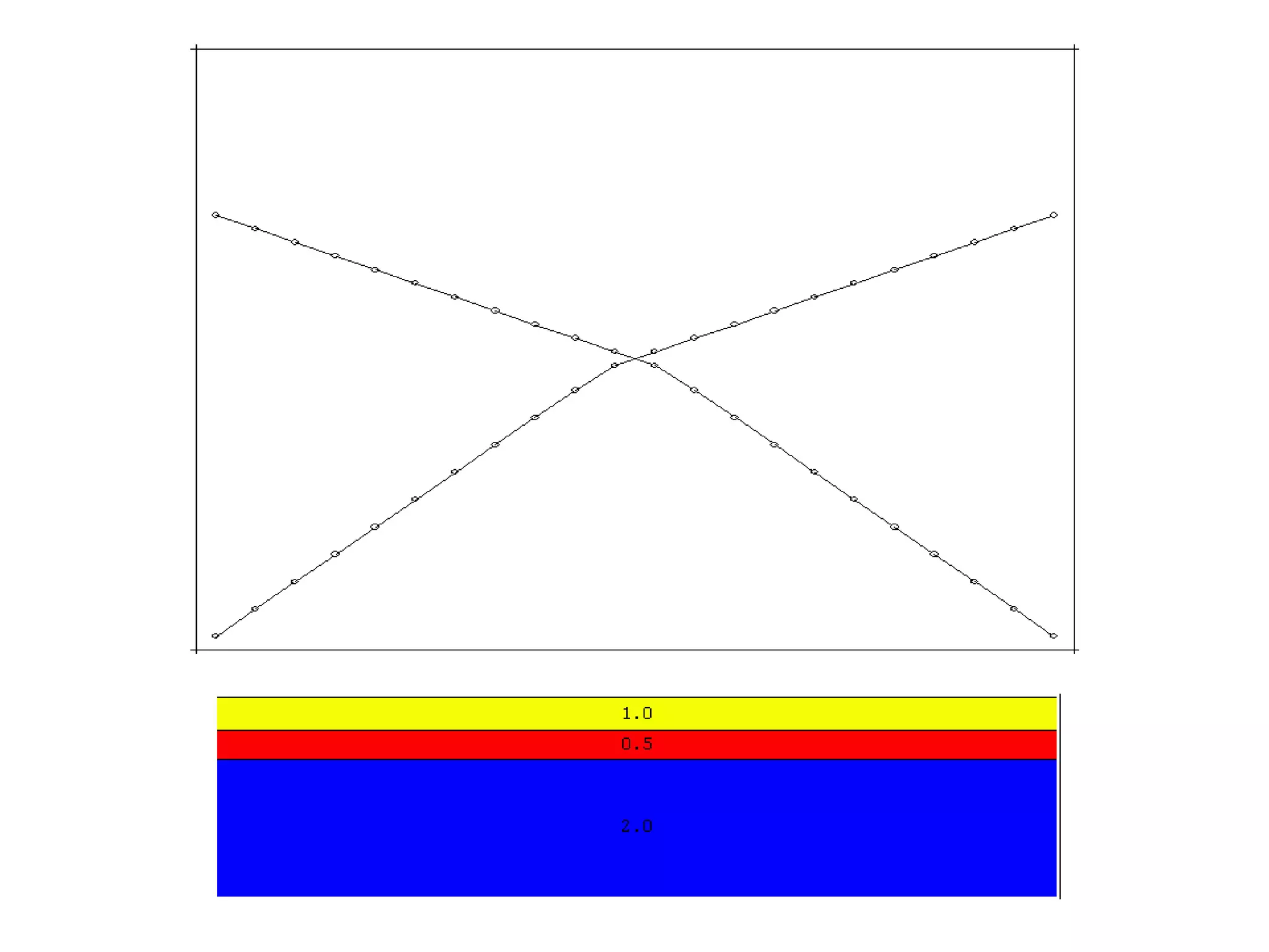
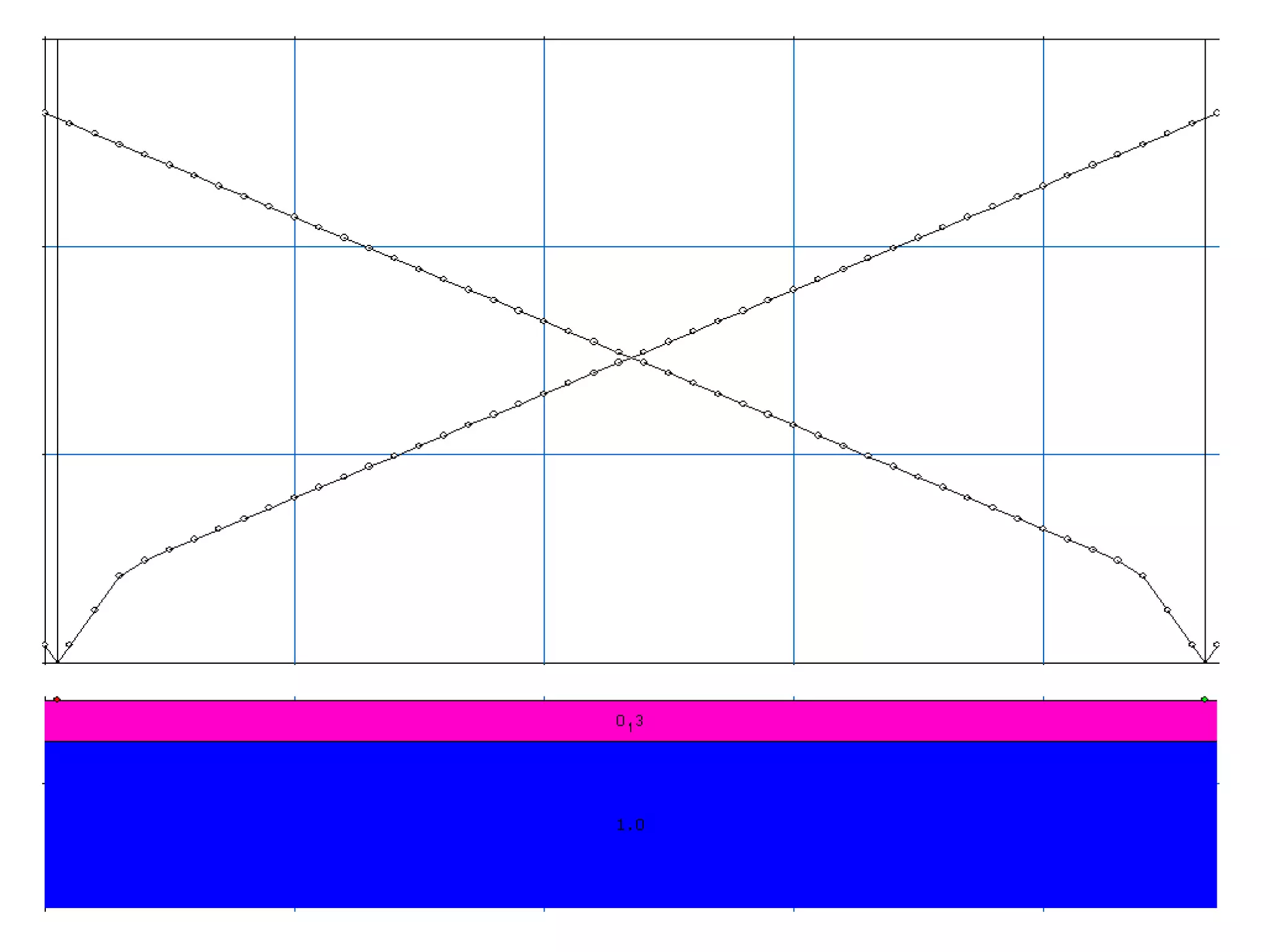
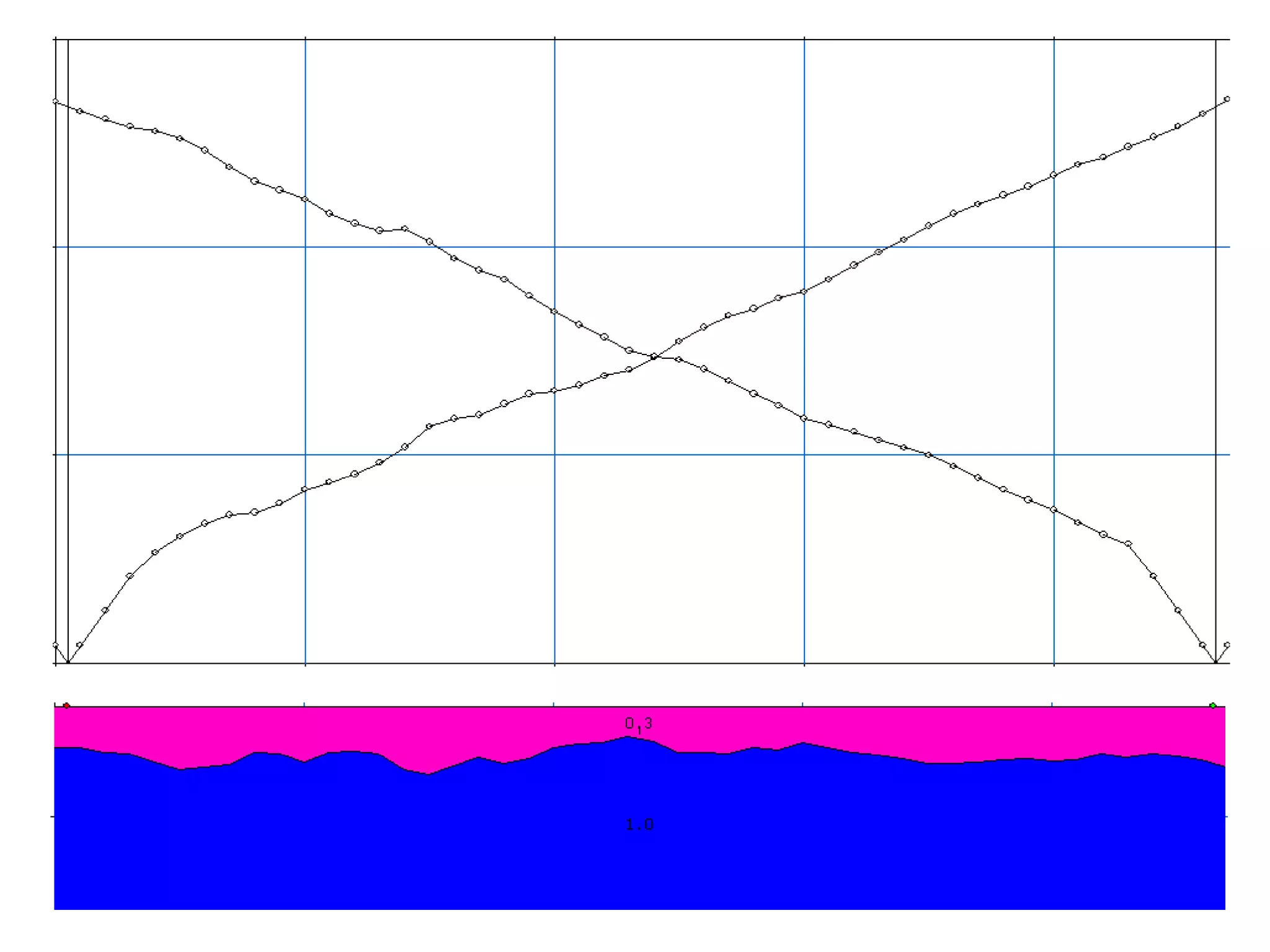
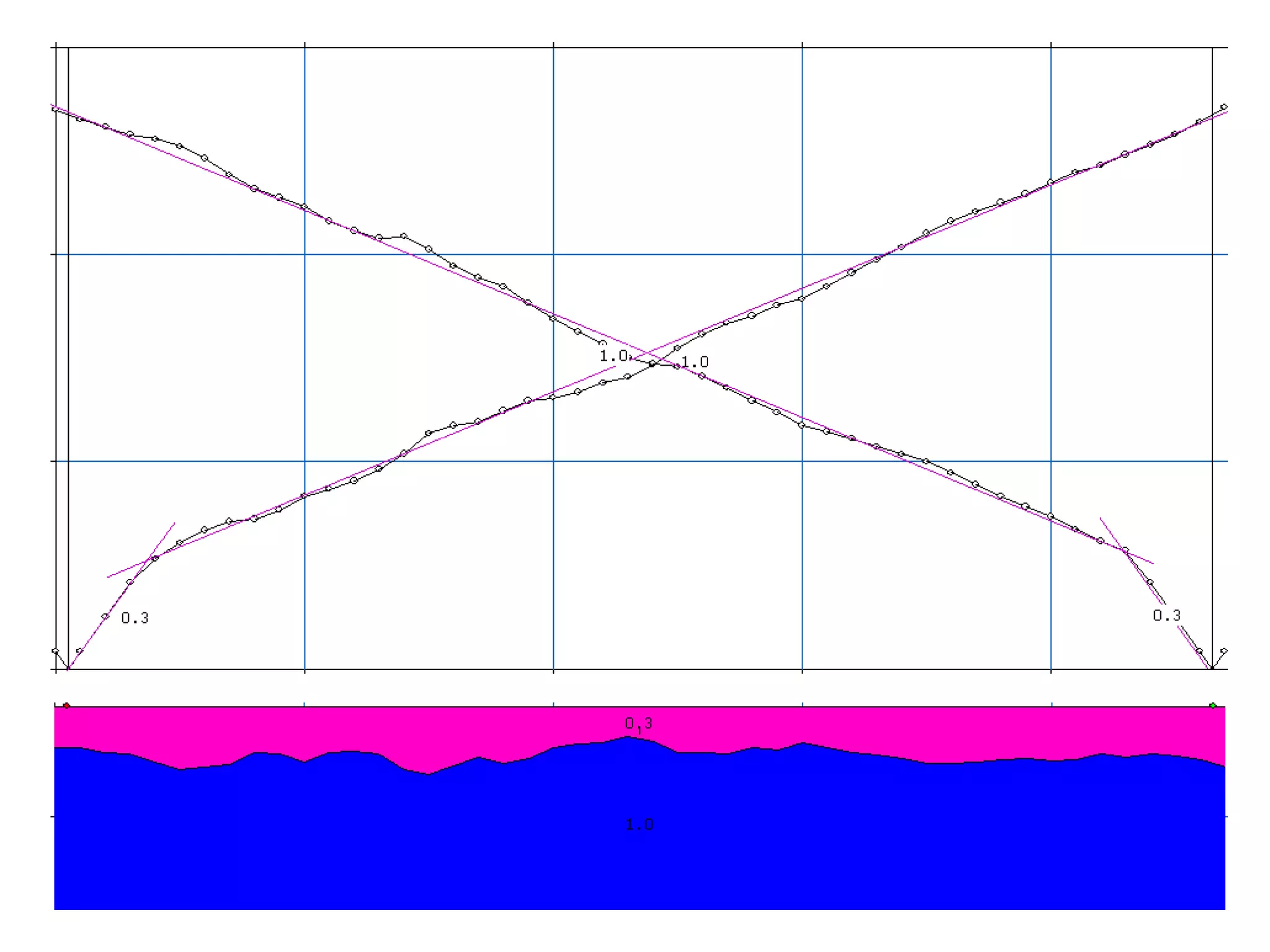
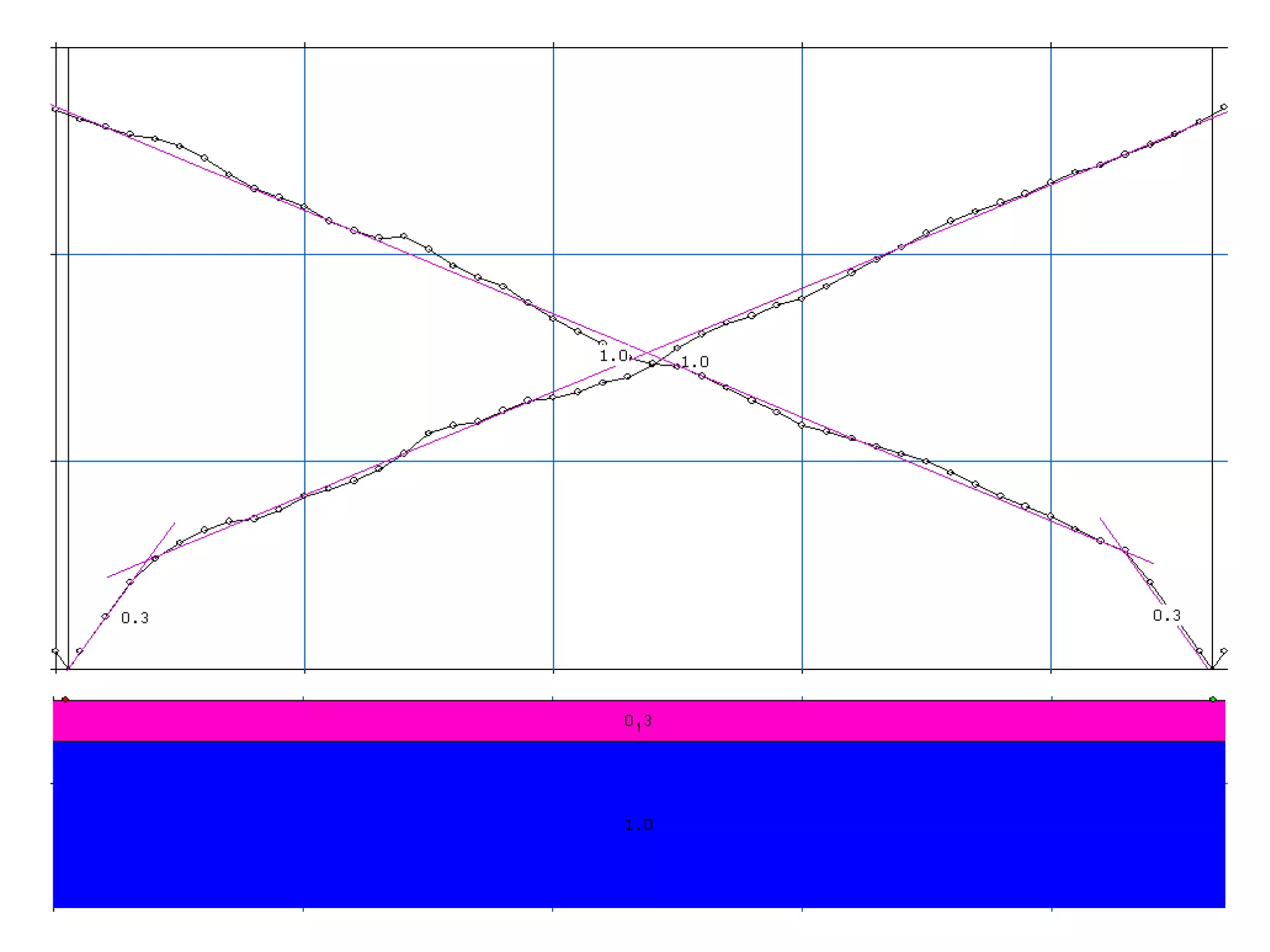
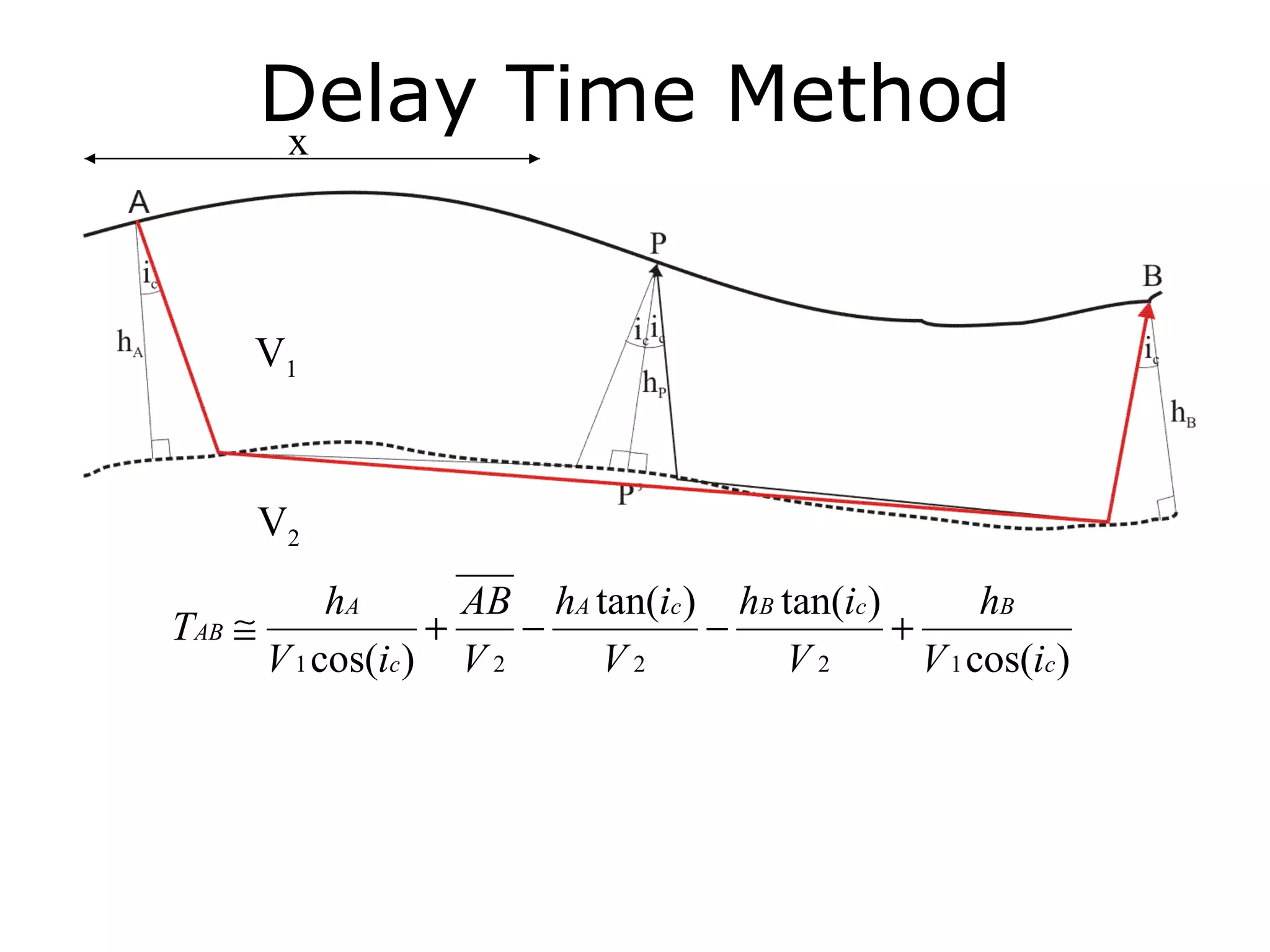
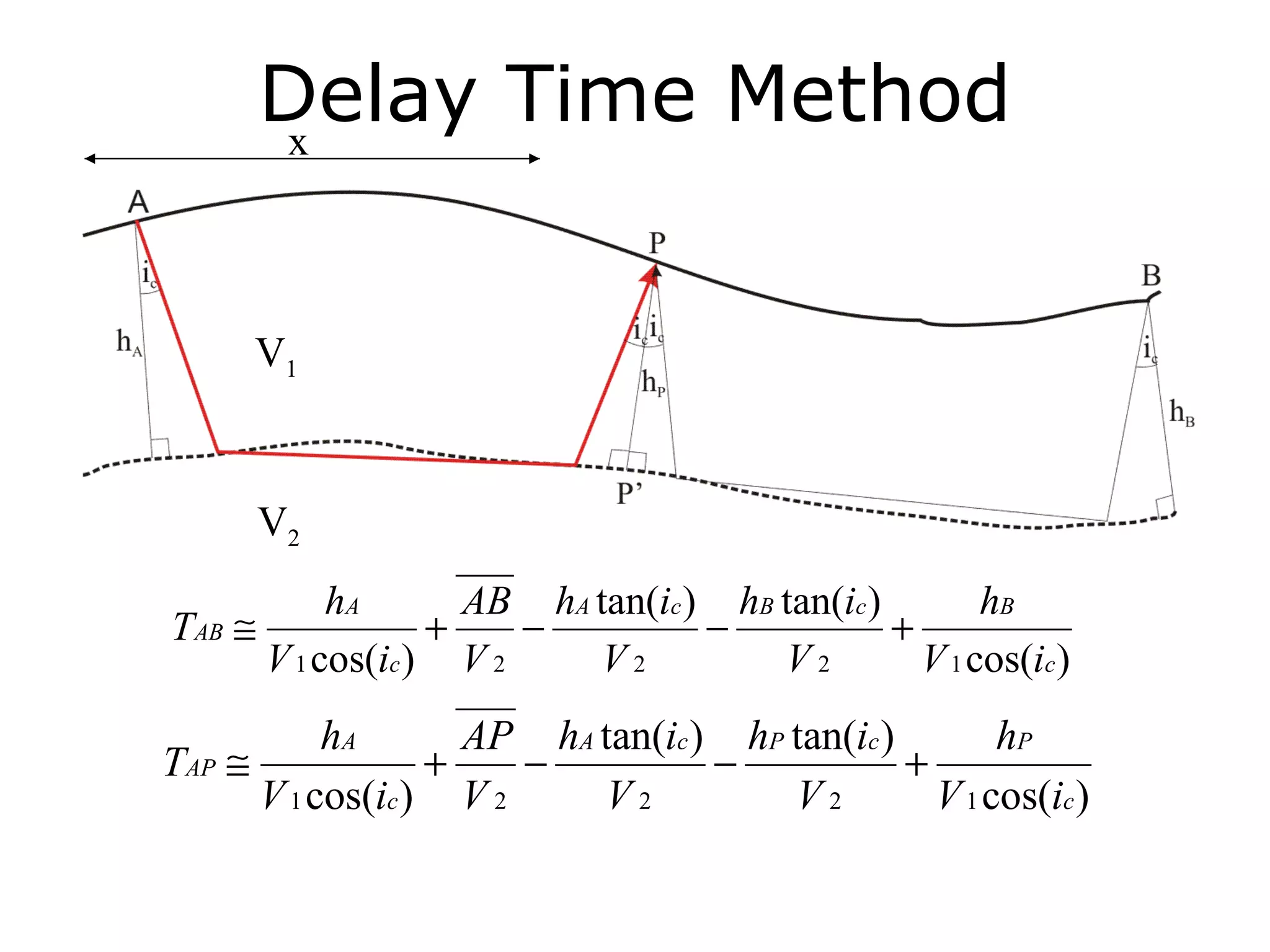
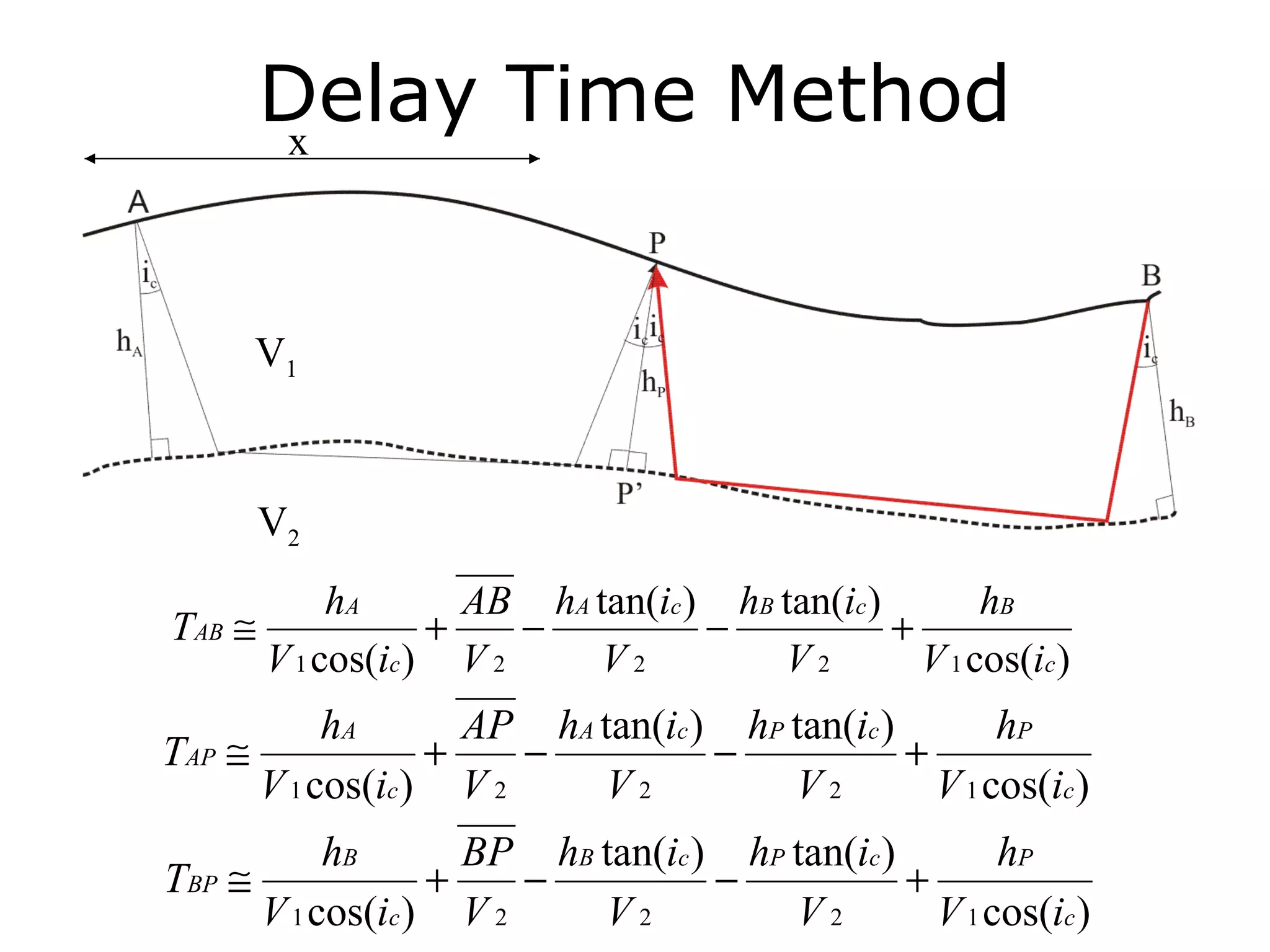
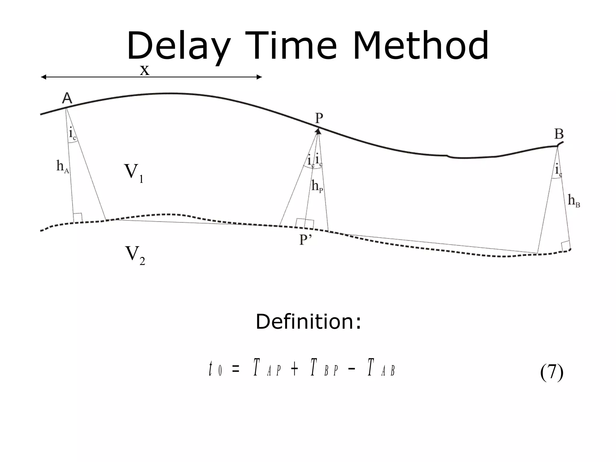
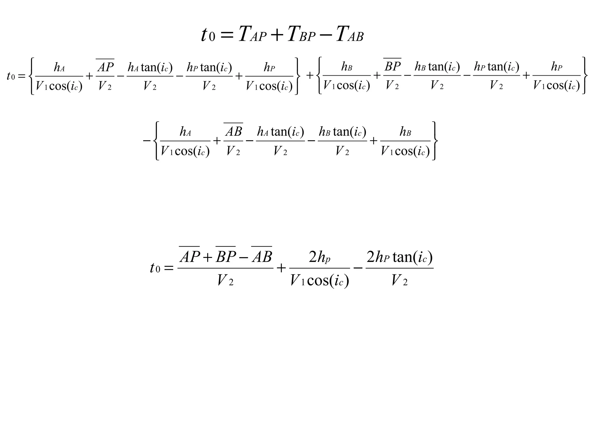
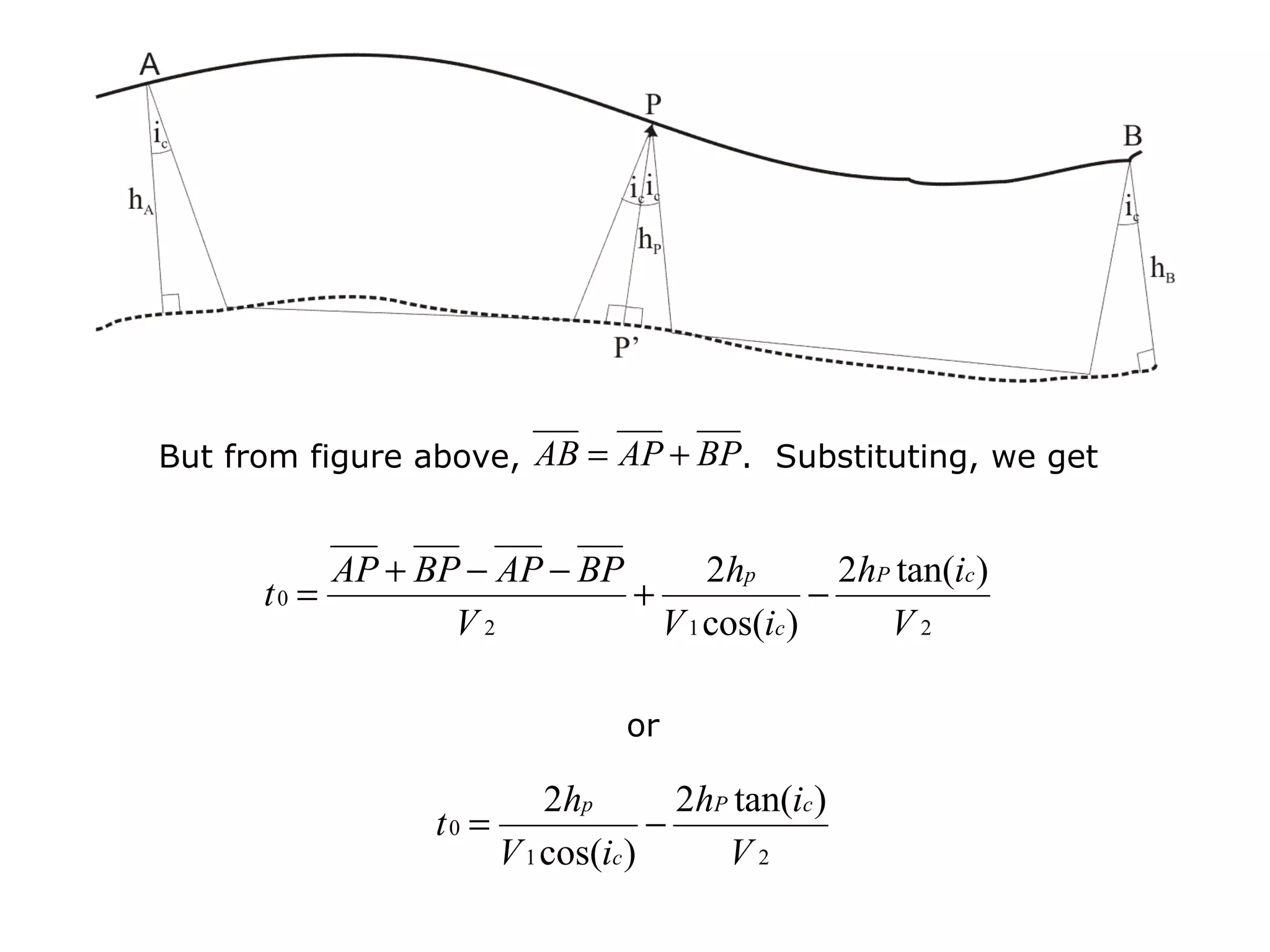
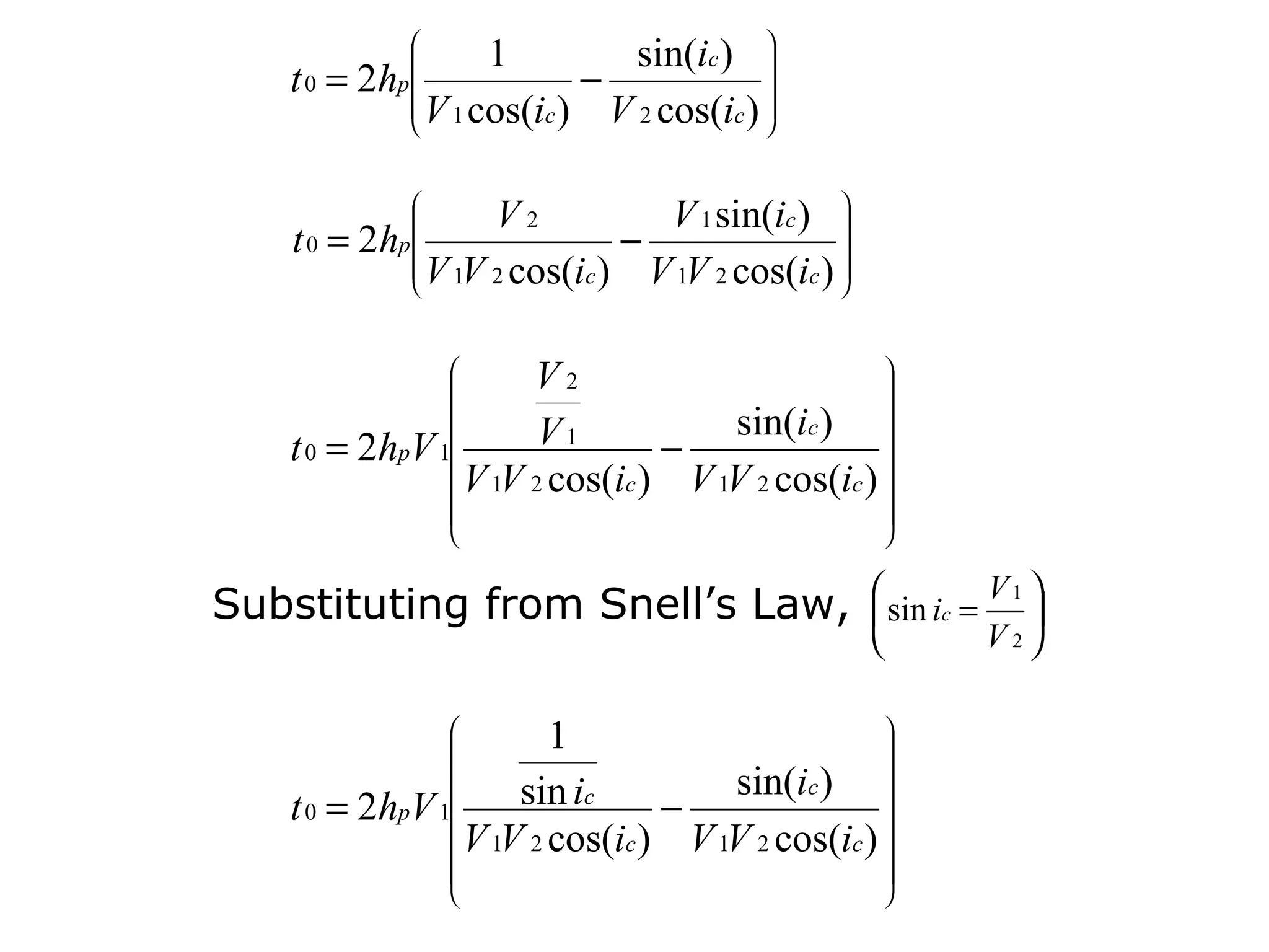
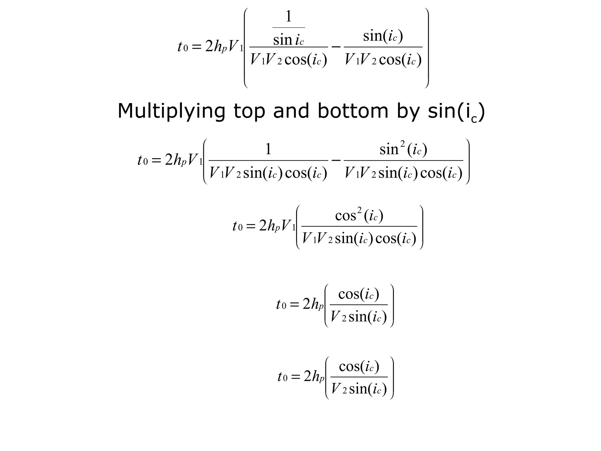

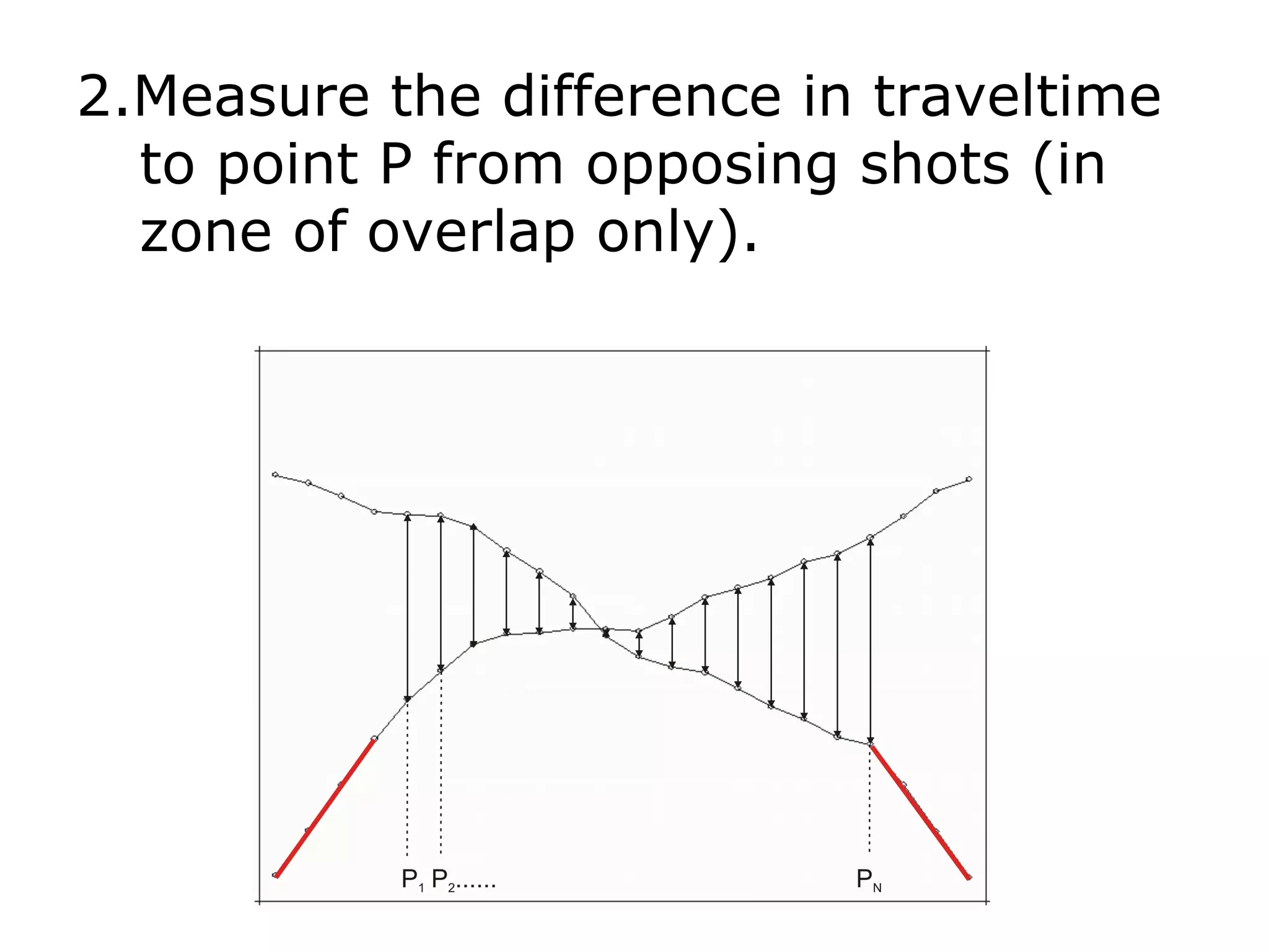
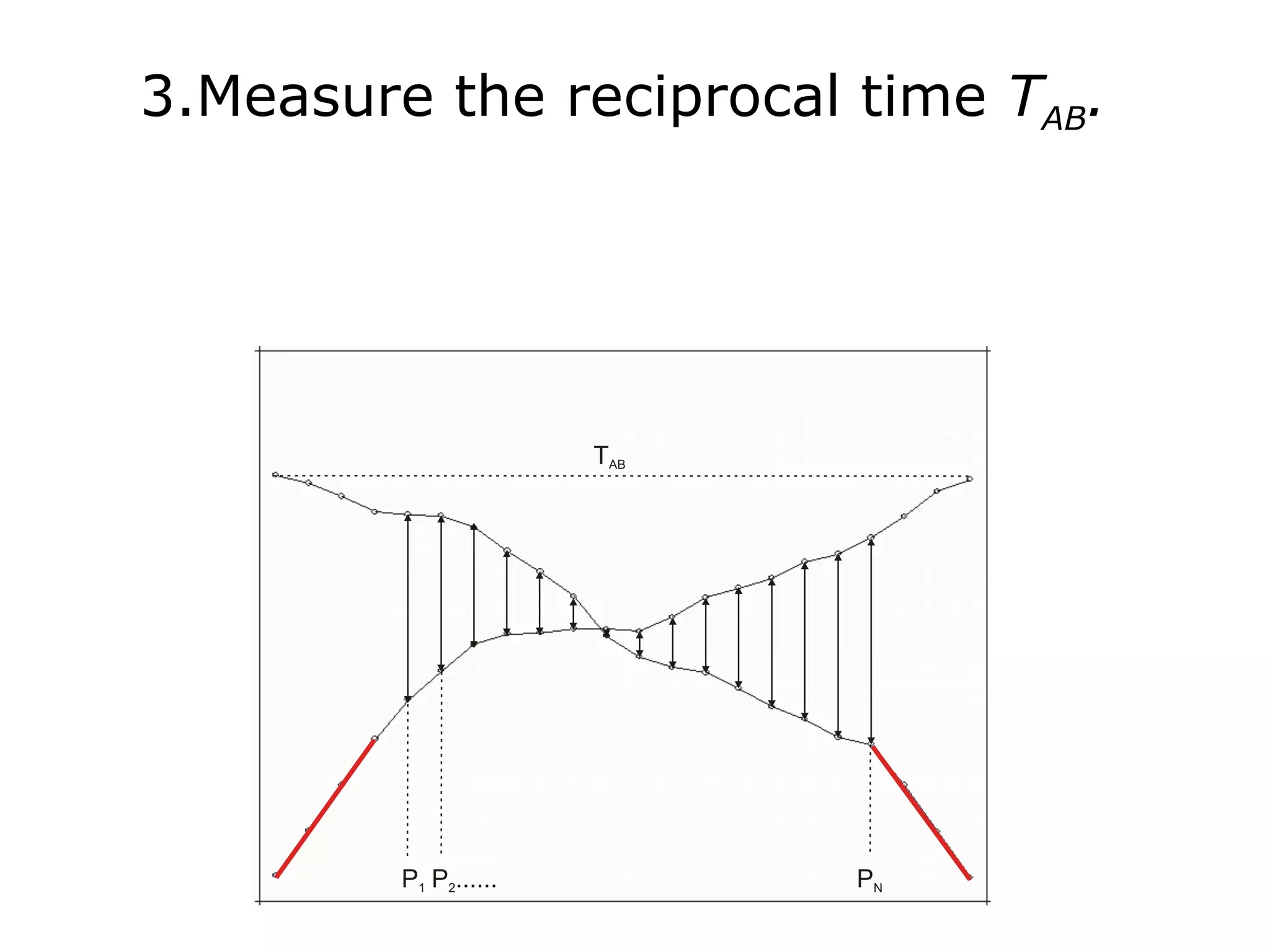
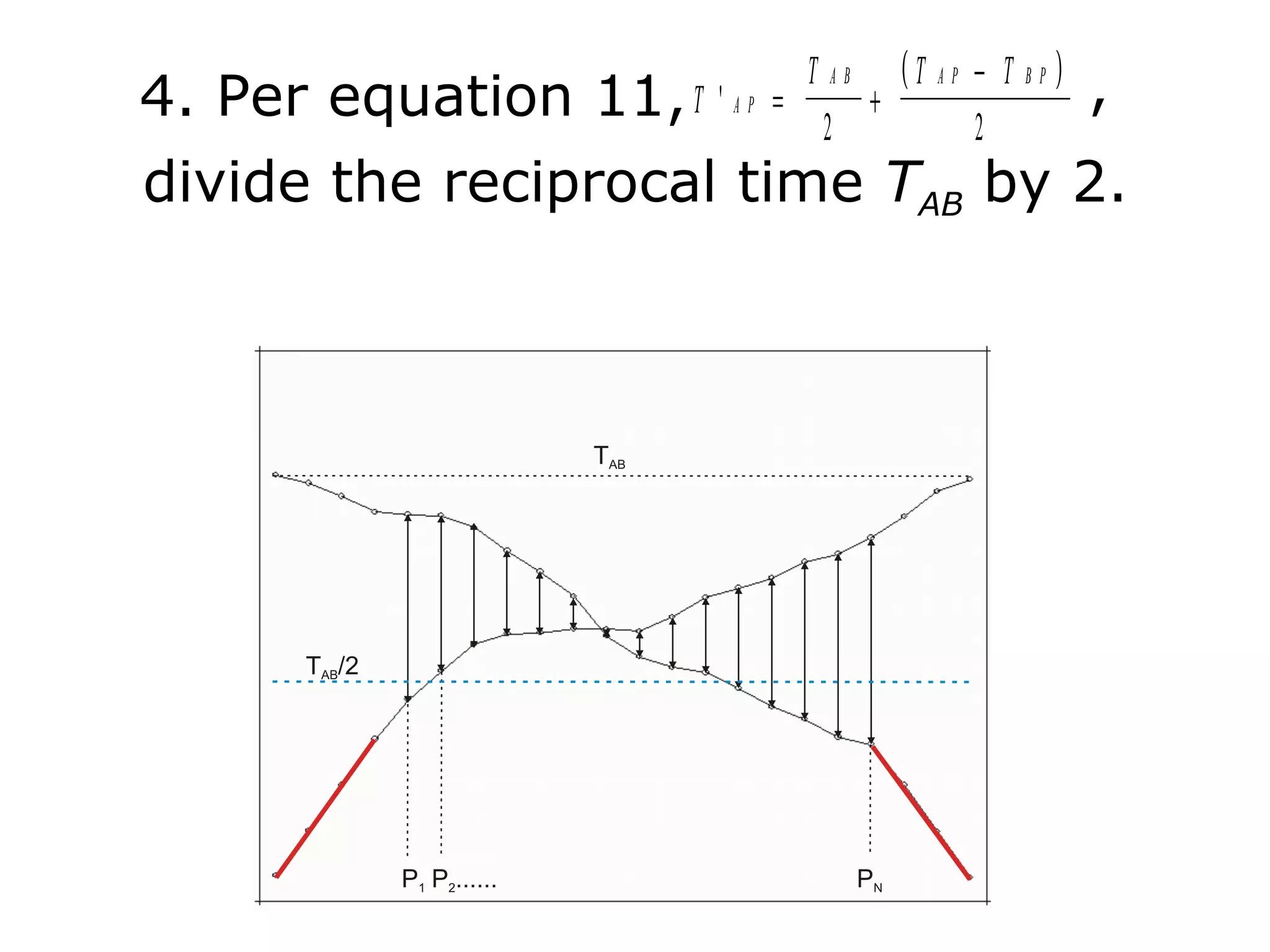
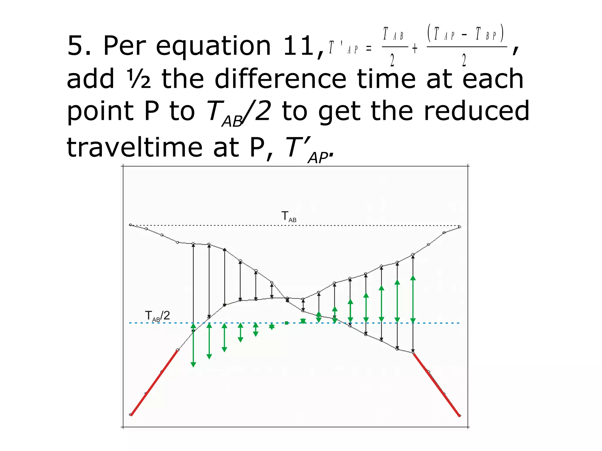
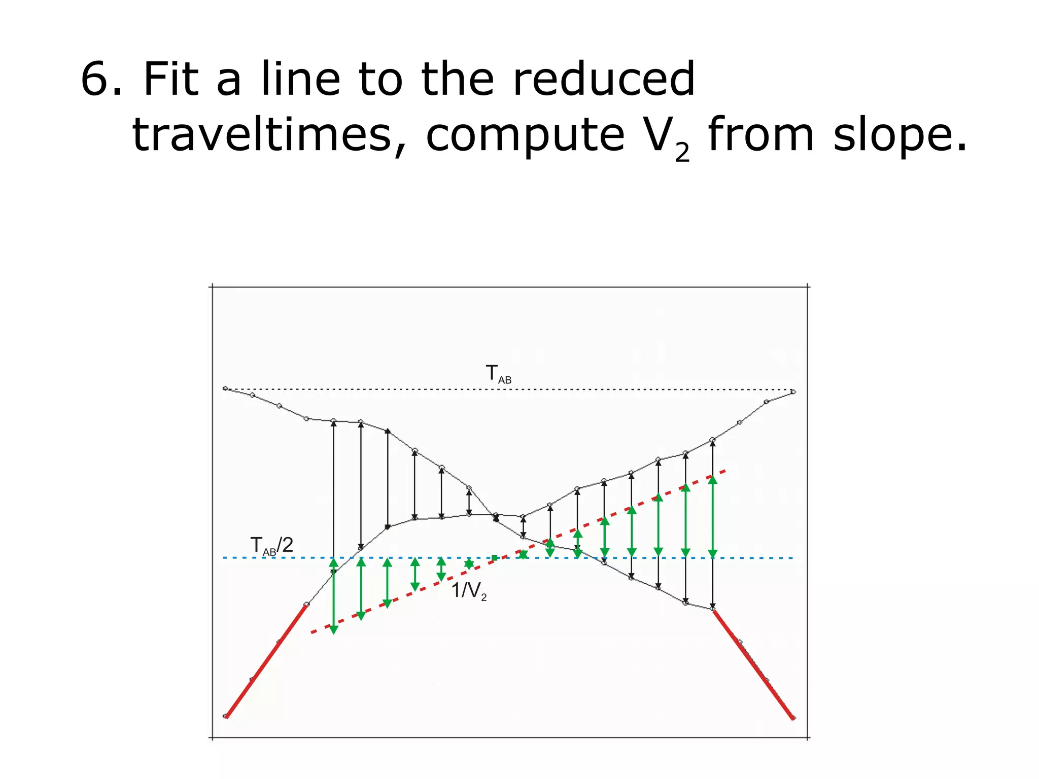
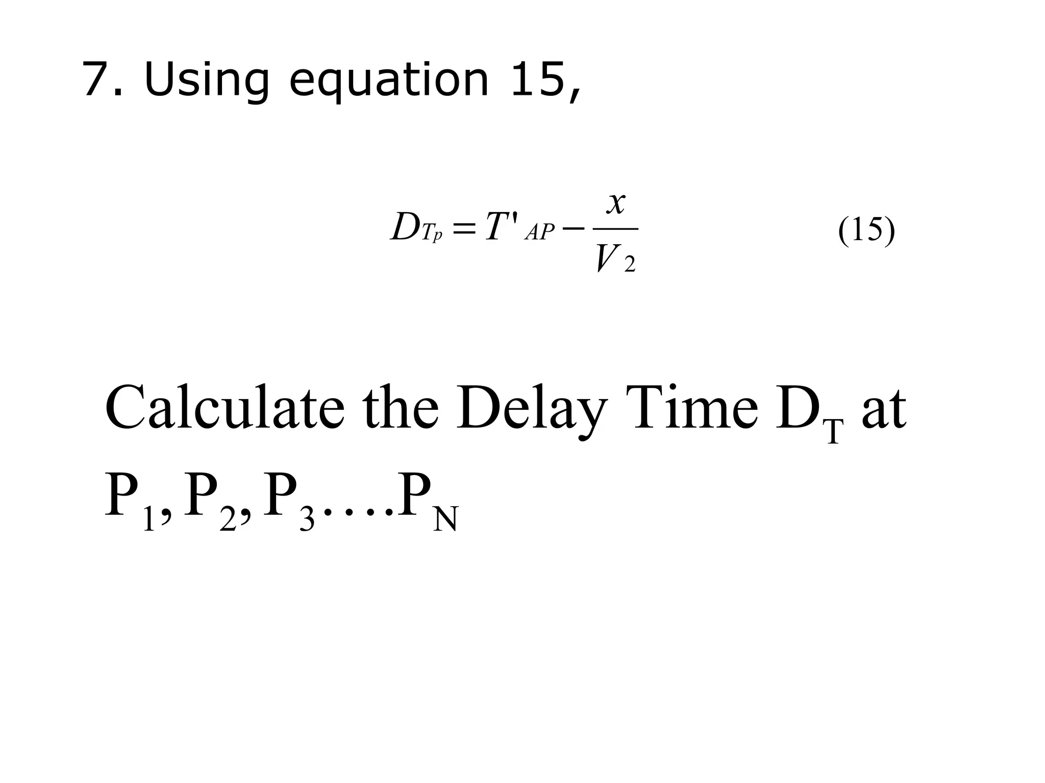
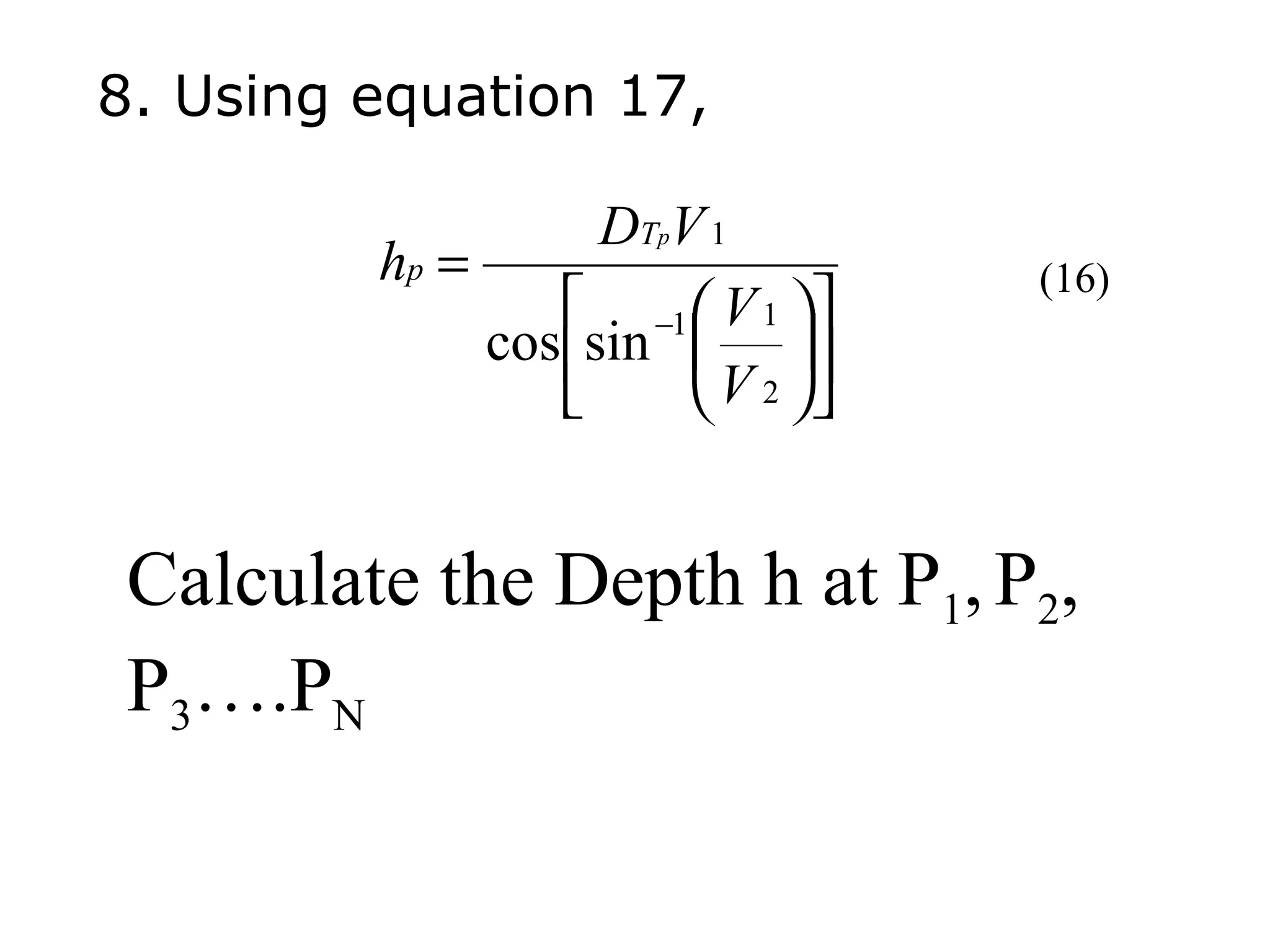


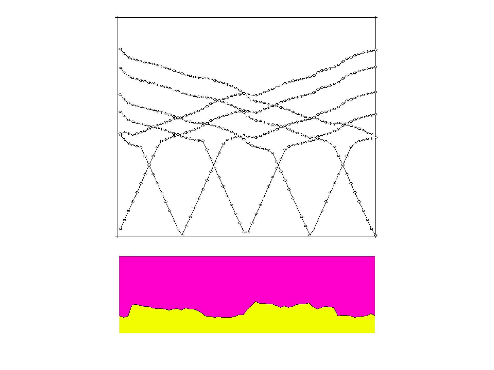
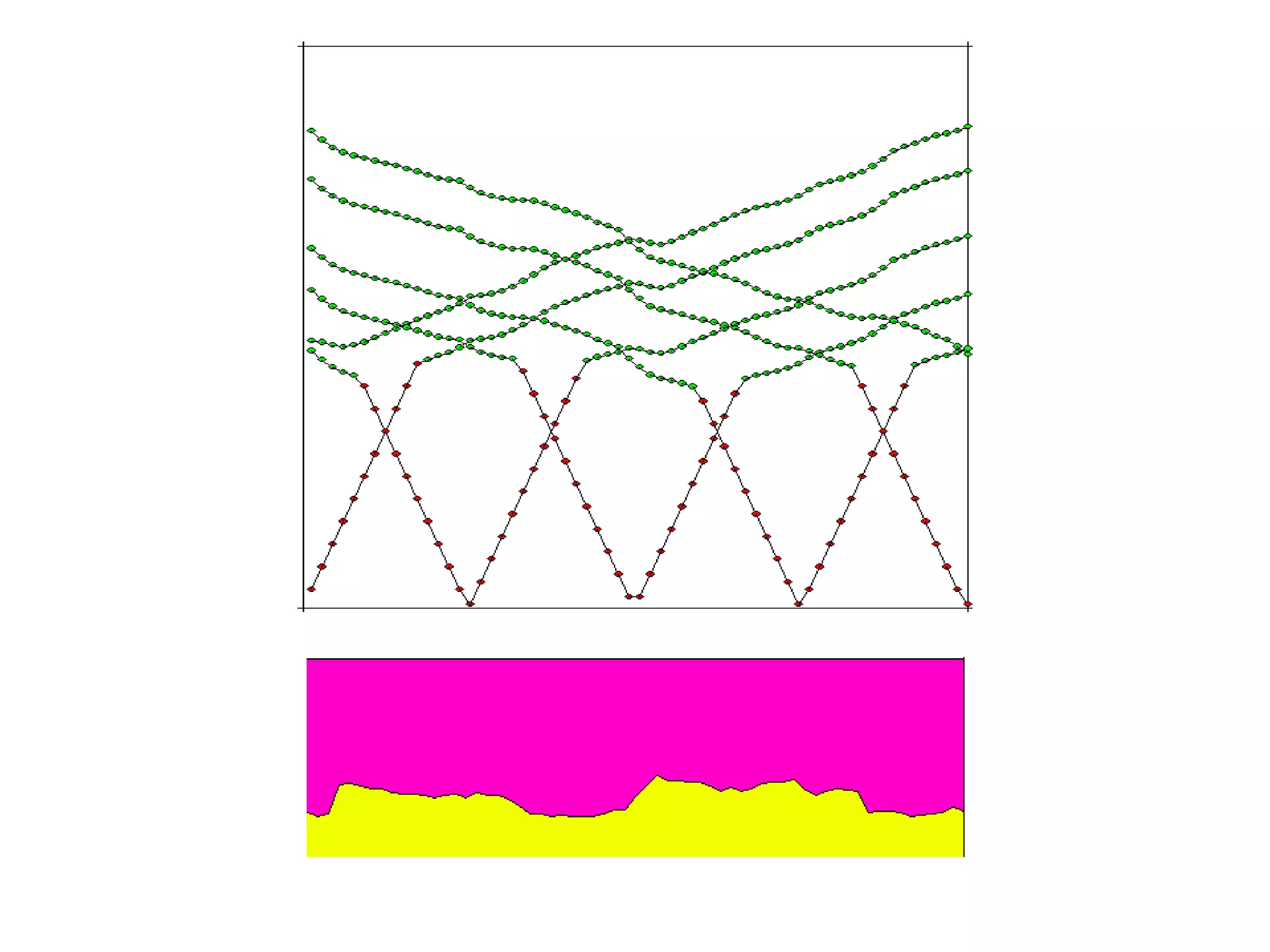
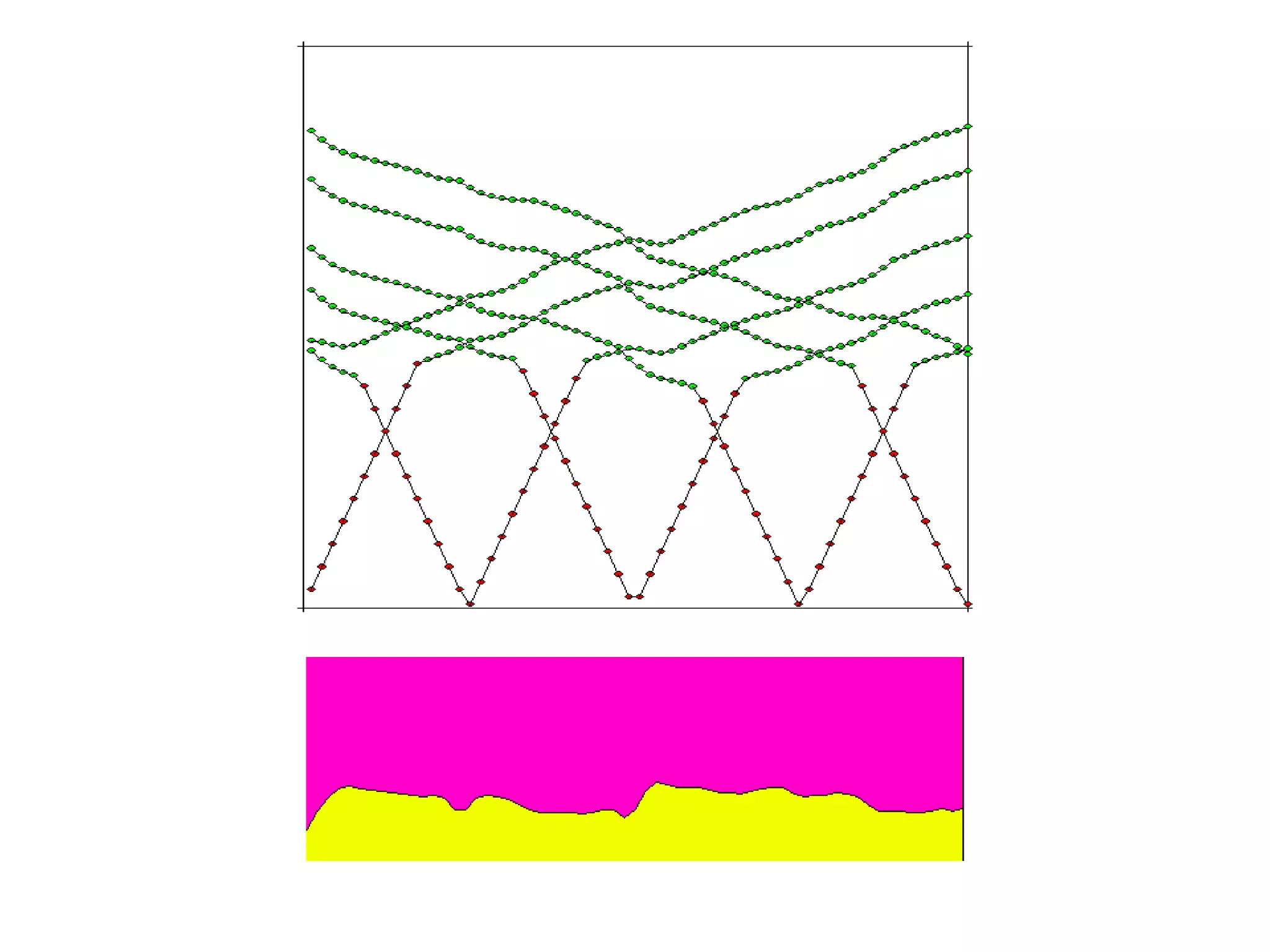
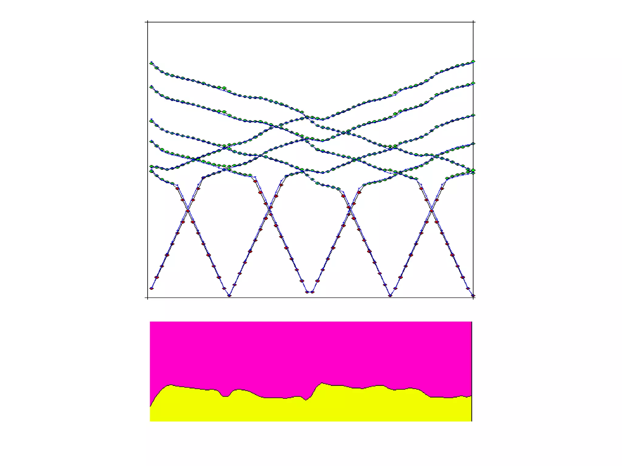
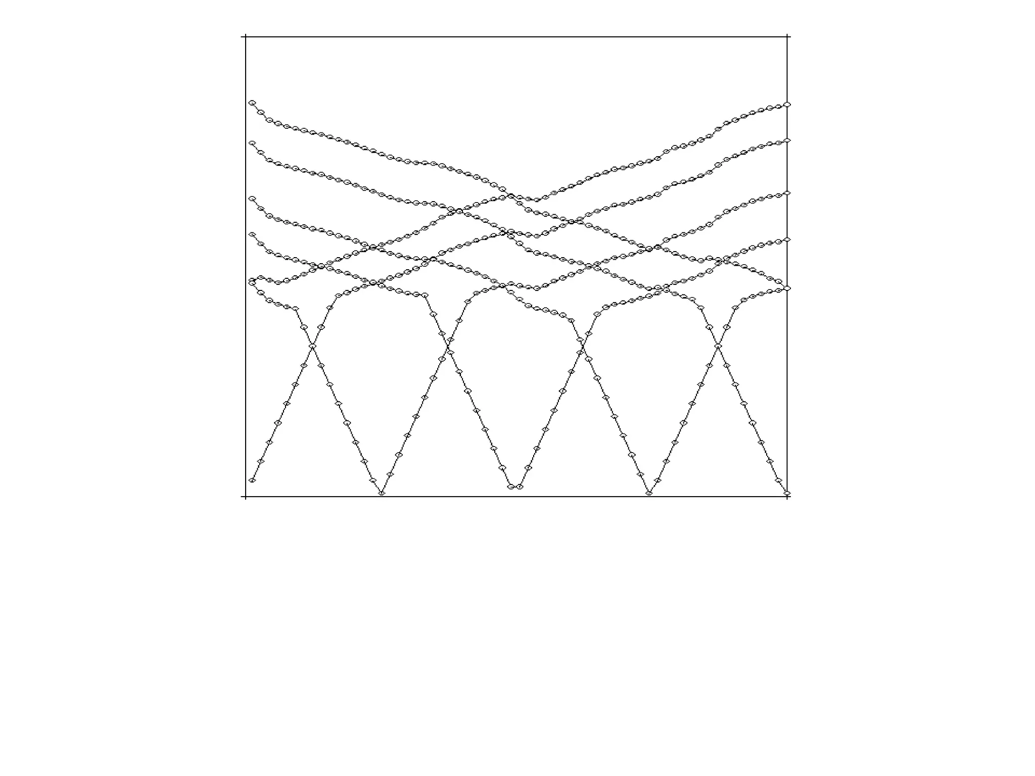
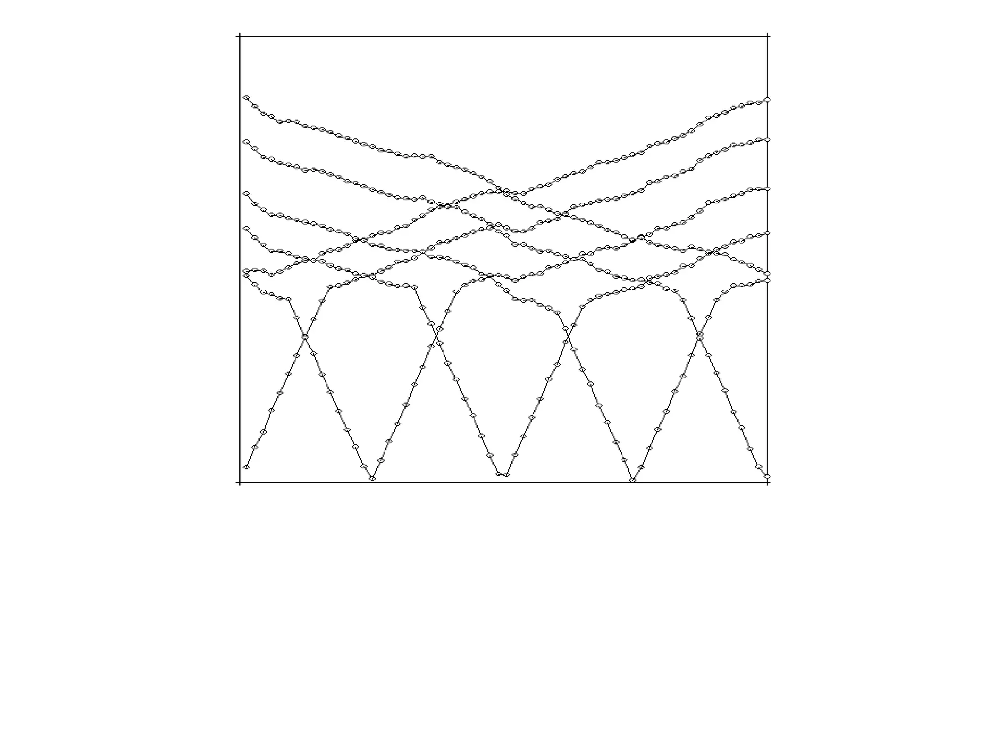
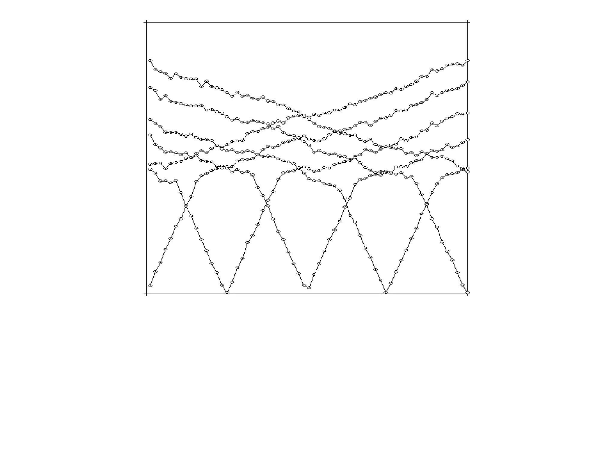
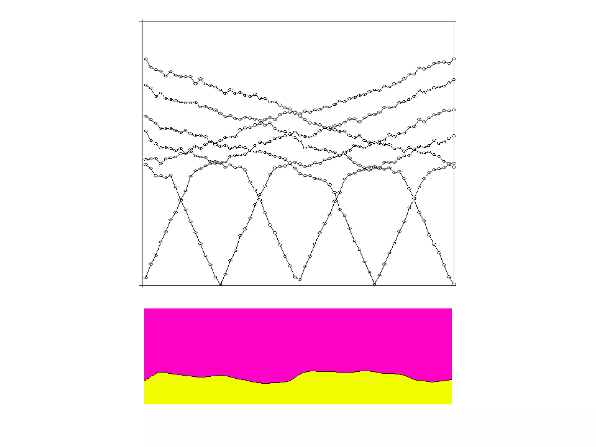

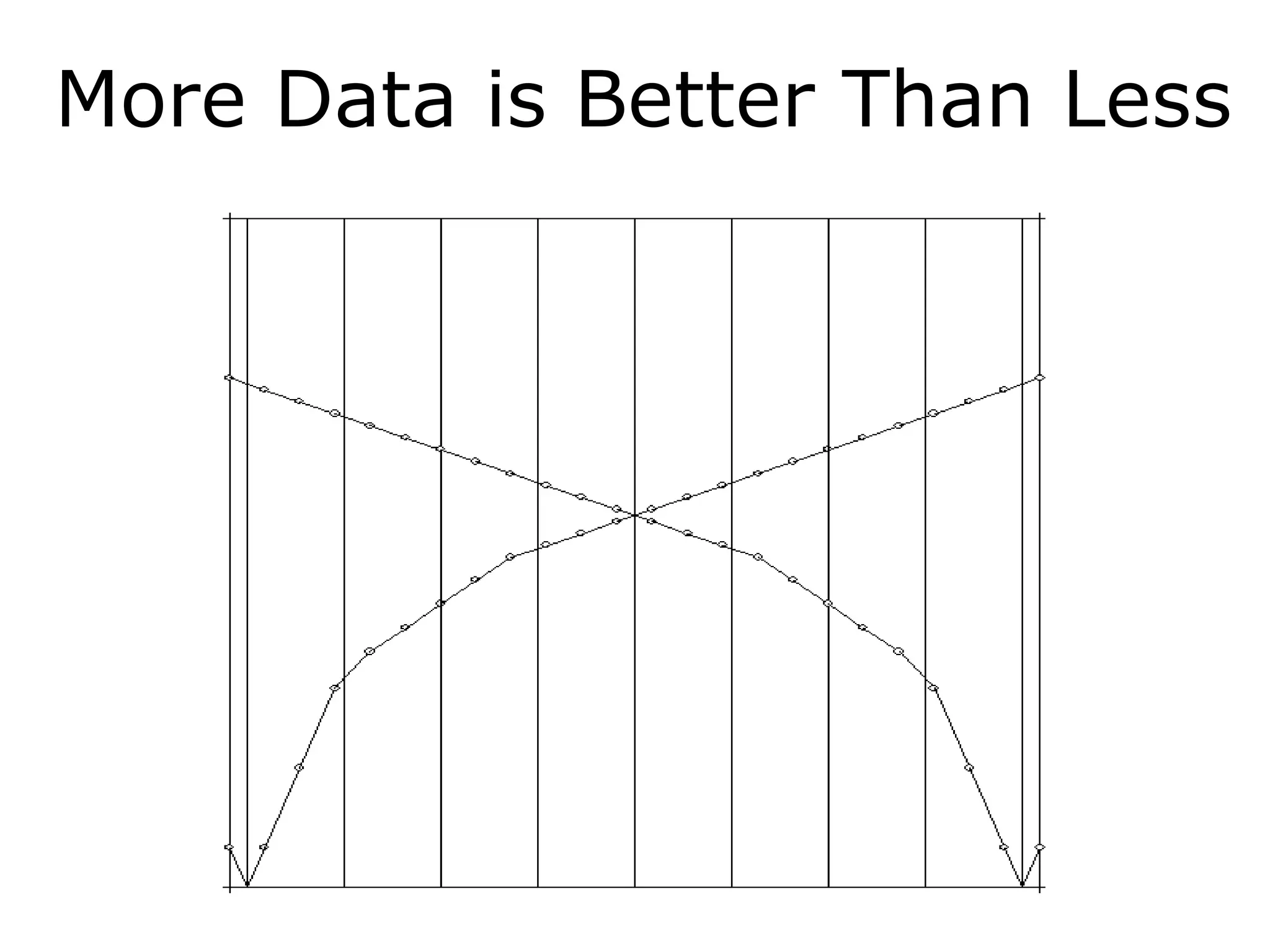
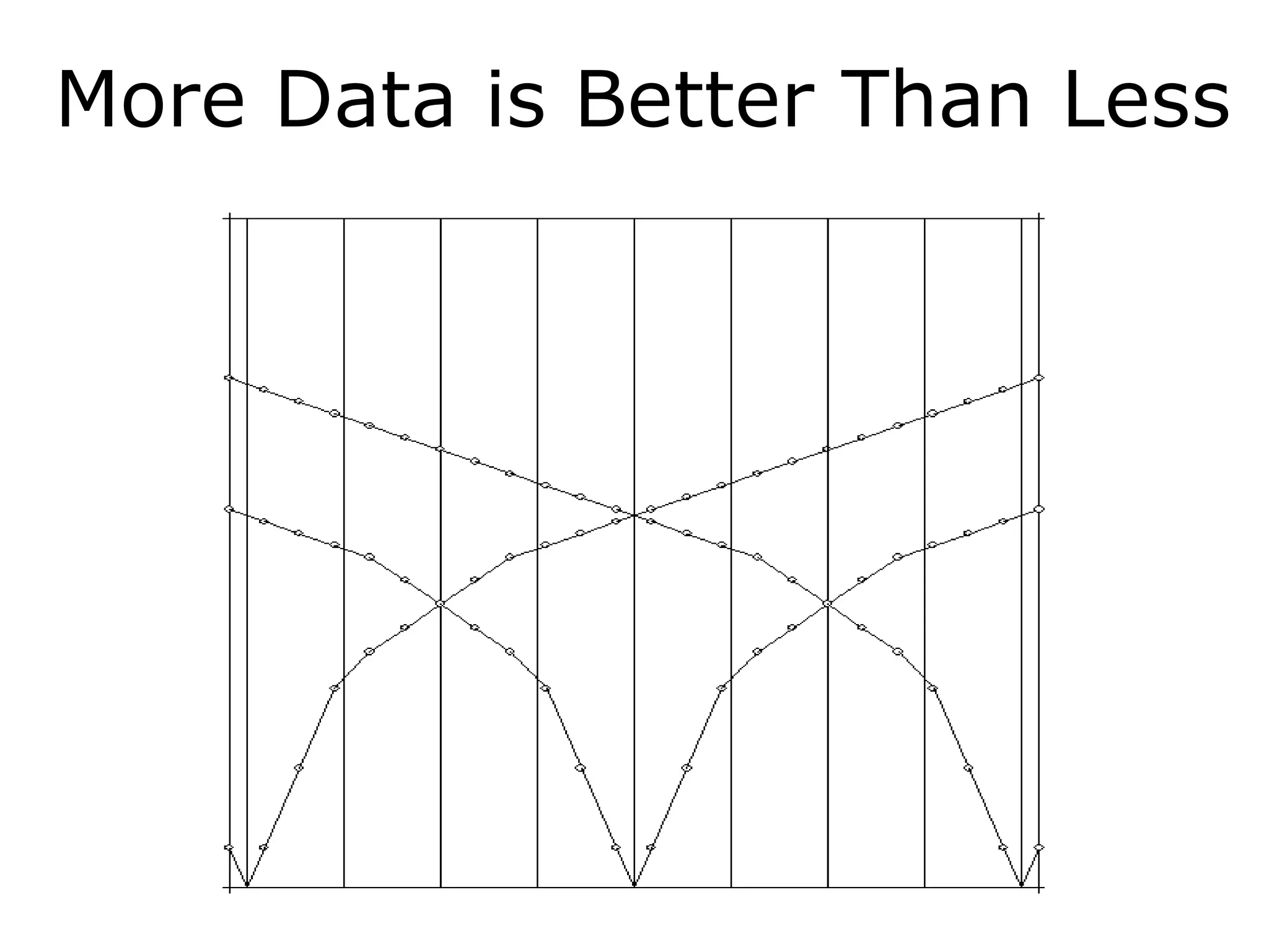
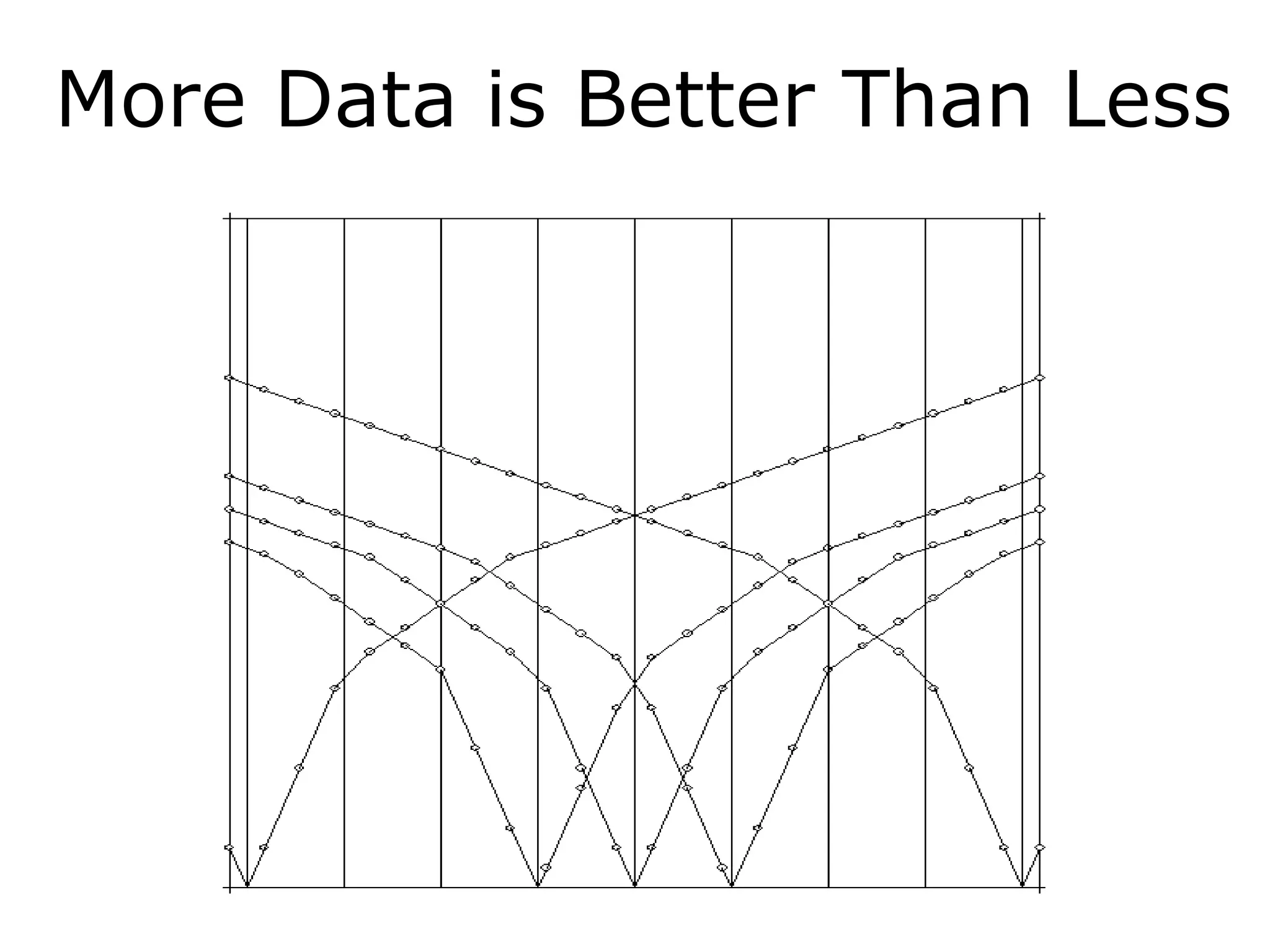
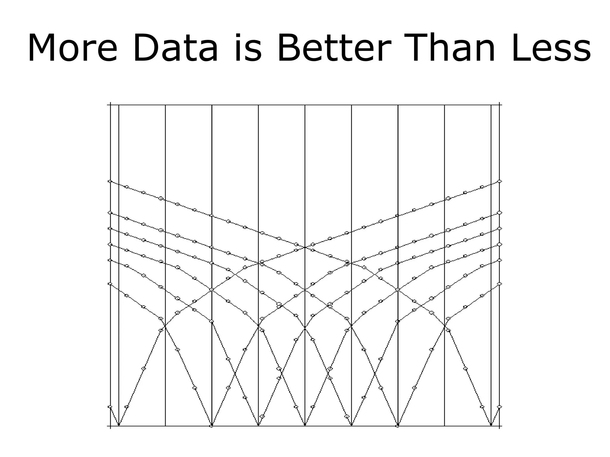
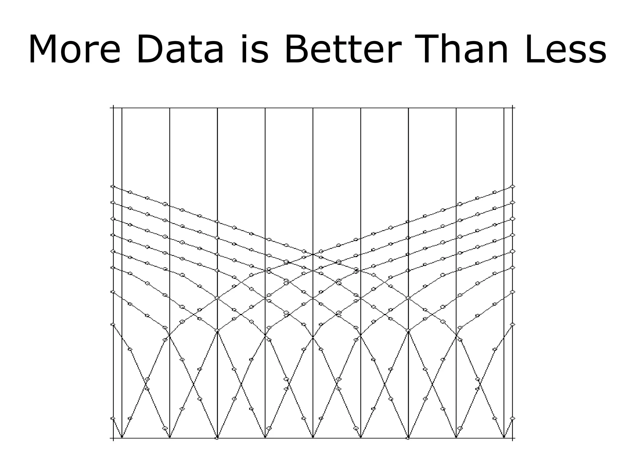
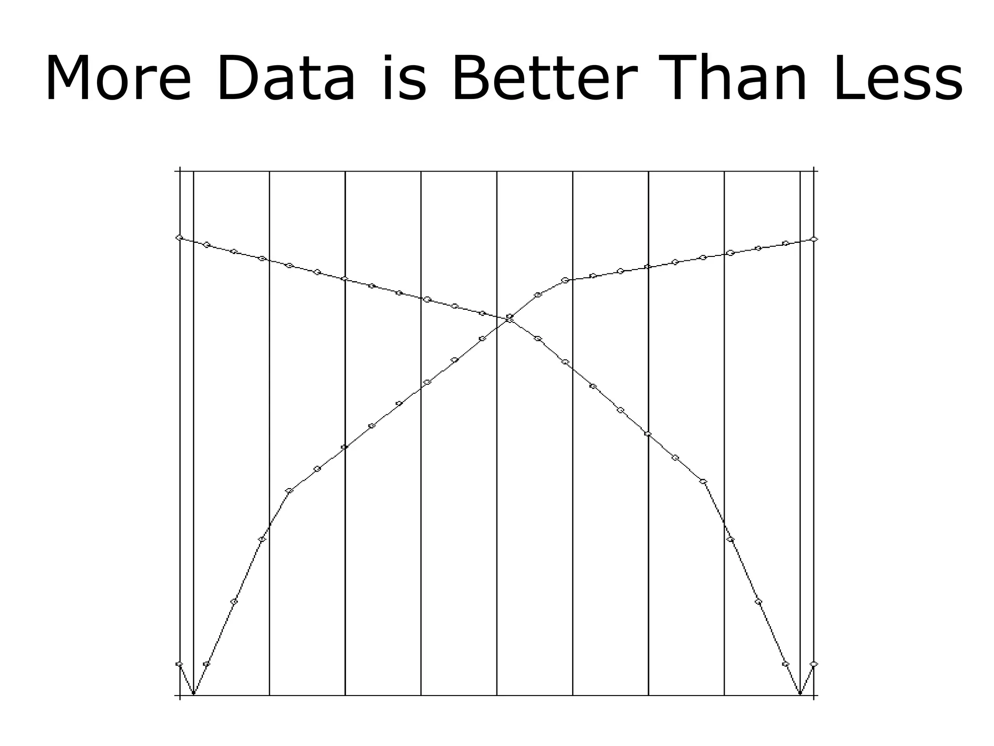
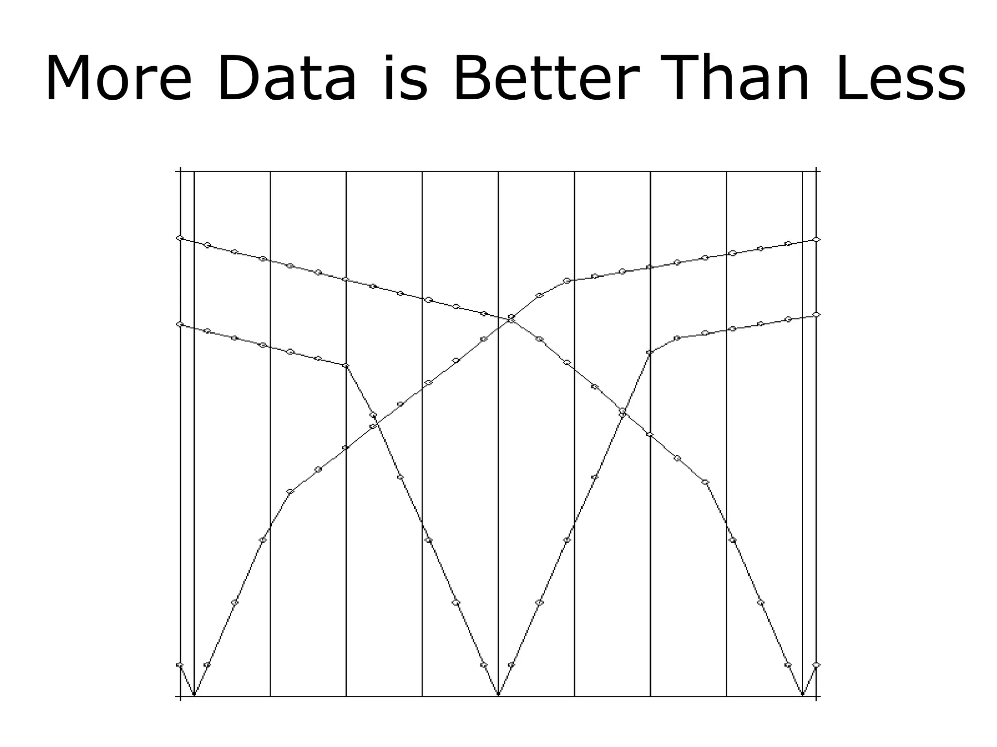
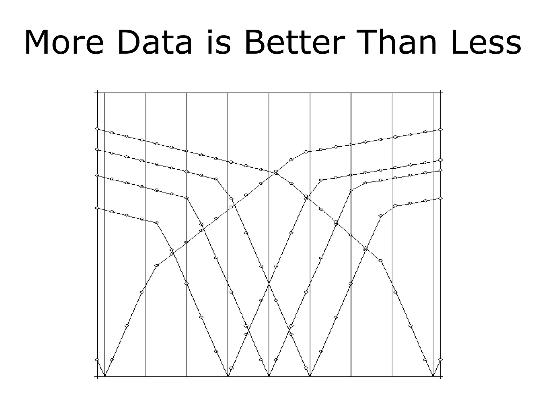
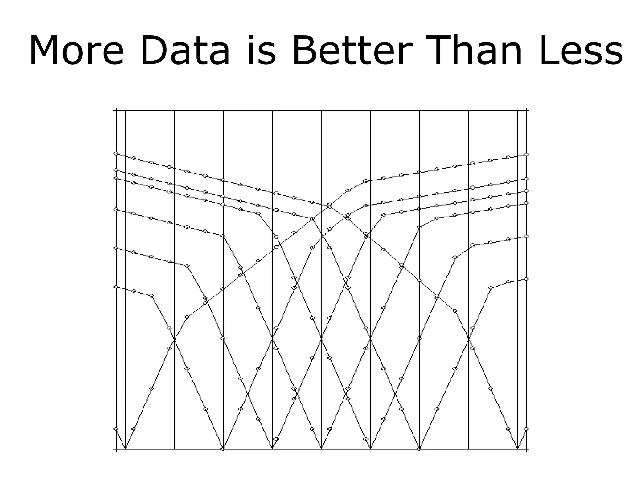
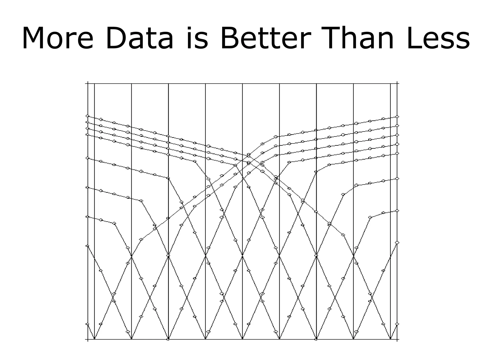
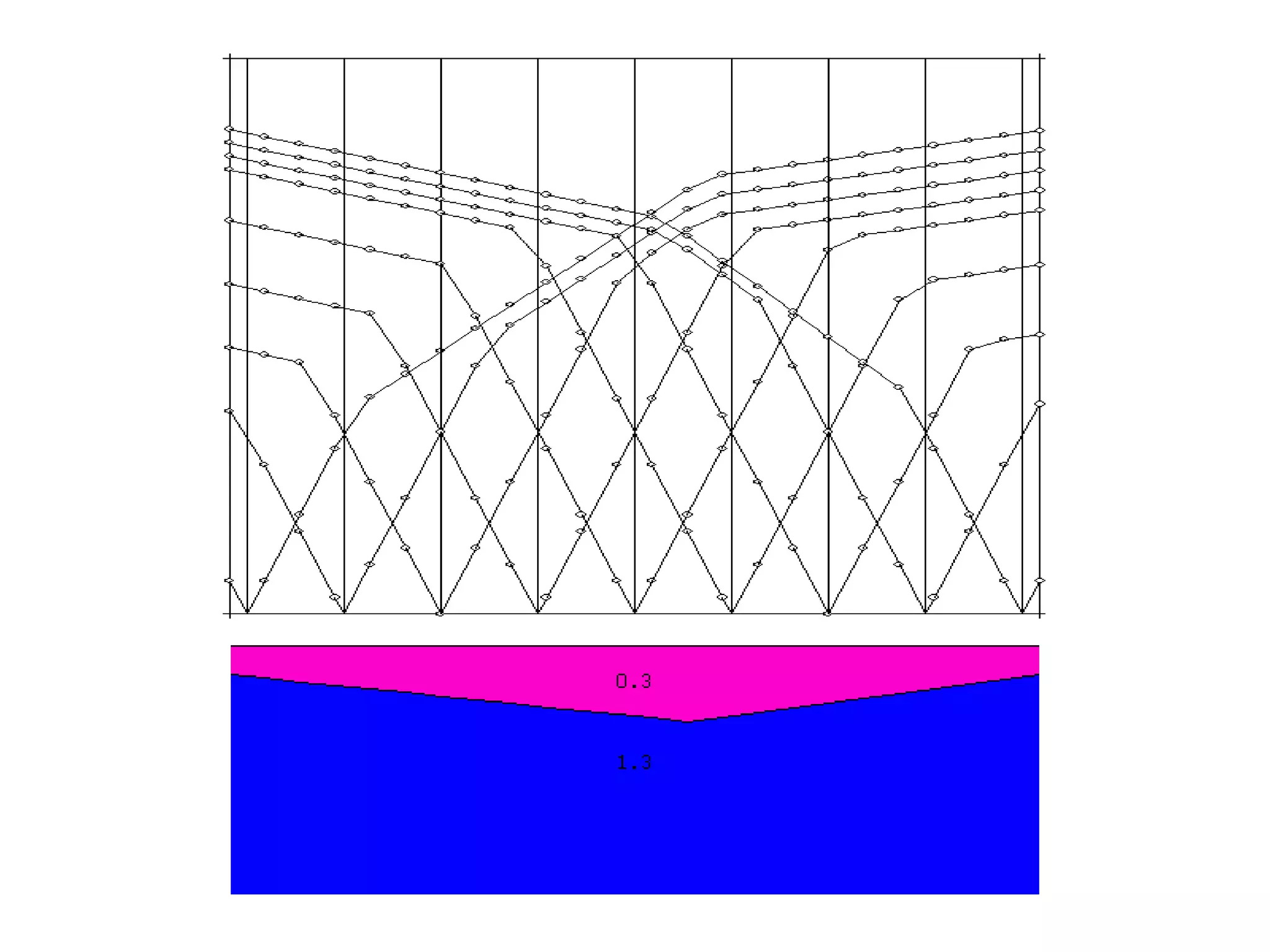

Geometrics, Inc. is a seismic equipment company located in San Jose, California. The document discusses fundamentals of seismic waves including particle motion, velocity, refraction, Snell's law, and how seismic refraction is used to map subsurface layers. Key equations are summarized that relate travel time, velocity, depth, and dip of layers. Dipping layers and velocity inversions are also addressed.


![Friction (2) [compatibility mode]](https://cdn.slidesharecdn.com/ss_thumbnails/friction2compatibilitymode-100415053857-phpapp01-thumbnail.jpg?width=640&height=640&fit=bounds)
![Friction [compatibility mode]](https://cdn.slidesharecdn.com/ss_thumbnails/frictioncompatibilitymode-100415053915-phpapp01-thumbnail.jpg?width=640&height=640&fit=bounds)


