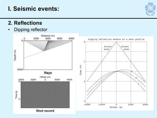
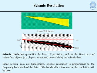
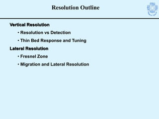
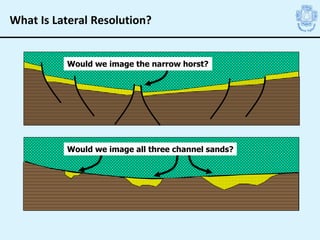
SlideShare a Scribd company logo
1 of 128
Md. Sakawat Hossain
DGS, JU, BD
Seismic Method
Courtesy of ExxonMobil
Mitchum et al., 1977b
AAPG©1977 reprinted with permission of the AAPG
whose permission is required for further use.
Courtesy of ExxonMobil
Basic Exploration Workflow
To D/P
Drop
Prospect
Drill
Wildcats
Confirmation
Well
Identify
Opportunities
Process
Seismic Data
Capture
Prime Areas
Interpret
Seismic Data
Acquire
Seismic Data
Success
Success
Failure
Uneconomic
Economic
Analysis
Assess
Prospects
• Seismic data shows edges of geologic units
• Edge detection that responds to AI changes
• AI = acoustic impedance = velocity*density
Seismic is a risk-reducing technology.
Oil is found by drilling, seismic reduces risk of -
• Dry holes
• Marginal producers
• Reserve estimate errors
General Concepts: Why seismic?
The seismic method can provide best subsurface image in exploration.
Seismic Acquisition
2D or 3D seismic survey is designed based on:
– Imaging Objectives: image area, target depth, dips, velocity,
size/thickness of bodies to be imaged, etc.
– Survey Parameters: survey area, fold, offsets, sampling,
shooting direction, etc.
– Balance between Data Quality & Cost of Survey
Land Operations
Vibrators Generate a Disturbance
Geophones Detect Motion
Marine Operations
Air Guns Generate a Disturbance
Hydrophones Detect Pressure
What is Seismology?
Recall 3rd year
The scientific discipline that is concerned with the study of earthquakes and of the propagation of
seismic waves within the Earth.
Application:
Exploration and engineering seismology deals with the use of elastic waves to map the
structure of the subsurface.
It mainly applies to
Hydrocarbon
Exploration
Reservoir characterization
Geo-engineering
Site characterization
Contamination remediation
Ore deposits
Hydrogeology
Archaeology
CO2 storage monitoring
Seismology
• Q: What is it that causes a seismic wave to reflect?
– A: Contrasts in acoustic impedance (at vertical incidence)
• Q: What happens as a seismic wave crosses a velocity
interface?
– A: Reflection and refraction (Snell’s Law)
• Q: How do seismic waves lose energy in the ground?
– A:
• Geometrical spreading
• Absorption
• Partitioning at interfaces
• Scattering
• Earth is a low-pass filter
Quick answer: Basic seismic theory
Seismic cartoon
Courtesy of ExxonMobil
Listening Devices 0 s

An Explosion! 0 s
Energy
Source .1 s
.2 s
.3 s
Some Energy is Reflected
Most Energy is Transmitted
.4 s
.4 s .5 s
Some Energy is Reflected
Most Energy is Transmitted
.6 s
.7 s
.8 s
.8 s
Seismic Methods
Device
#1
Device
#2
0.0
0.3
0.4
0.5
0.6
0.7
0.8
0.1
0.2
For the explosion we just considered ...
Listening device #1 records a reflection
starting at 0.4 seconds
Listening device #2 records a reflection
starting at 0.8 seconds
To Image the Subsurface, We Use Many Shots (explosions)
and Many Receivers (listening devices or Geophone)
Arranged in Lines either on Land or Offshore
Time
Raw Seismic Data
• Half-space
– Two-layer Earth
– Boundary is the free surface
• Direct arrivals
– Air wave/Ground roll
– Direct wave
• Travel time is linear
I. Seismic events:
1. Direct arrivals
• Half-space
• Estimate velocity from seismic
data
– Plot of time vs distance (x-t space)
– Velocity is slope of curve
I. Seismic events:
1. Direct arrivals
I. Seismic events:
1. Direct arrivals
I. Seismic events:
• Beyond half-space, layer can introduce below the surface
– In x-t space, reflection is hyperbolic curve
– Hyperbolic moveout (or normal moveout)
I. Seismic events:
2. Reflection
I. Seismic events:
2. Reflection
•Horizontal reflector - Reflection point is midpoint on surface
• Dipping reflector - Reflection point is no longer midpoint on surface
I. Seismic events:
2. Reflection
• Dipping reflector
I. Seismic events:
2. Reflections
Layer Thickness
1 10 20
20
ms
30
base
top top
*
Seismic Resolution
Seismic resolution quantifies the level of precision, such as the finest size of
subsurface objects (e.g., layers, structures) detectable by the seismic data.
Since seismic data are bandlimited, seismic resolution is proportional to the
frequency bandwidth of the data. If the bandwidth is too narrow, the resolution will
be poor.
Seismic Resolution
Frequency, ƒ = 1/T
Unit of Frequency (ƒ), Hz
Unit of Period (T), s
The period (T) is the duration of
time of one cycle in a repeating
event, so the period is the reciprocal
of the frequency.
The frequency (ƒ) of a wave
describes the number of complete
cycles which are completed during
a given period of time.
The bandwidth describes simply the
breadth of frequencies comprising a
spectrum (e.g. 10-20 Hz)
Vertical Resolution
• Resolution vs Detection
• Thin Bed Response and Tuning
Lateral Resolution
• Fresnel Zone
• Migration and Lateral Resolution
Resolution Outline
II. Detection vs. Resolution - Analogy
You are driving at night.
You spot a light in the distance.
Is it a car or a motorcycle???
Aha, it is a car!
Detection: Ability to identify that some feature exists
• Detection limit is always smaller than the resolution limit
• Detection limit depends upon Signal-to-Noise
Resolution: Ability to distinguish two features (vertically or
horizontally) from one another
II. Detection vs. Resolution - Analogy
What is the minimum vertical distance between two
subsurface features such that we can tell them
apart seismically?
Shale
Sand
Sd
Gamma Ray
Shale
Baseline
For Example:
Based on seismic data,
could you determine that
there is a thin shale layer
between the two sands?
II. Vertical resolution
Applying the concept of resolution to seismic
wiggles, vertical resolution quantifies the
resolvability of seismic waves along the direction of
wave propagation, which is usually the vertical
direction.
Hence it is also called temporal resolution, depth
resolution or 1D resolution, depending on the
application.
The smallest change in input that will produce a detectable change in output.
The ability to distinguish two points that are near each other.
The ability to localize an event seen through a window, usually taken as the half
width of the major lobe.
Four cases of vertical resolution defined by the detectability of two events close
together. (Lower) Richer’s resolution limit is the separation interval between
inflection points of the seismic wavelet.
II. Vertical resolution
Question: What is a thick bed?
Impedance Composite
Wavelet
1
R. C. Wavelet
2
NO
Interference
λ
Wavelet 1 ends before
Wavelet 2 begins
Top of Bed
Response
Base of Bed
Response
Answer: A thick bed is one that has a TWT > λ (pulse duration or Dp)
B
A
C
Thick Bed Response
Wavelet 1 ends before
Wavelet 2 begins, no
interference of wavelet
TWT thickness = 0.9 * Dp
Impedance Composite
Wavelet
1
R. C. Wavelet
2
Some
Interference
Wavelet 2 starts before
Wavelet 1 ends
Top of Bed
Response
Base of Bed
Response
2nd half-cycle from Wavelet 1
and 1st half-cycle from Wavelet 2
form a trough doublet
B
A
C
Dp
Partial Interference
TWT thickness = ½ Dp
Impedance Composite
Wavelet
1
R. C. Wavelet
2
Maximum
Interference
Wavelet 2 starts before
Wavelet 1 ends
Top of Bed
Response
Base of Bed
Response
2nd half-cycle from Wavelet 1
and 1st half-cycle from Wavelet 2
are completely in phase
resulting in 2x amplitude
B
A
C
Dp
Maximum Interference - Tuning
• Beds with reflection coefficients of equal magnitude
but opposite polarity
II. Resolution: Vertical
• Beds thicker than ½ wavelength are interference free. Beds between ½ and
¼ wavelength overlap and interfere constructively if the reflection coefficients
are of opposite sign
• Thus, the bed thickness is greater than one quarter of a wavelength (λ/4),
you have distinct reflections. Or, maximum constructive interference occurs
at 1/4 wavelength (tuning thickness).
II. Resolution: Vertical
• Amplitude decreases between 1/4 and 1/8 wavelength.
• Below 1/8 wavelength waveform shape is indistinguishable from that produces by
a single bed
• At about 1/30 l interference destroys the reflection no matter how large the
reflection coefficient
II. Resolution: Vertical
l/4
l/2
Single
Reflector
Wedge
Shallow Event (for example at 1 km depth)
Velocity = 2000 Meters / sec
Pulse:
Center Frequency = 50 Hz
Period = 1 / 50 = .020 sec
Wavelength = .020 x 2000 = 40 Meters
Limit of bed thickness to be detected (Tuning thickness)
= 40 /4 = 10 Meters
Deep Event (for example at 1.5 km depth)
Velocity = 3000 Meters / sec
Pulse:
Center Frequency = 20 Hz
Period = 1 / 20 = .050 sec
Wavelength = .050 x 3000 = 150 Meters
Limit of bed thickness to be detected (Tuning thickness)
= 150 / 4 = 37.5 Meters
II. Resolution: Vertical
Period
(ms)
wavelength =
period X velocity
Pulse
What Is Lateral Resolution?
Would we image the narrow horst?
Would we image all three channel sands?
What is the minimum horizontal distance between two
subsurface features such that we can tell them apart
seismically?
Reflections from Reflector with Gaps
Neidell & Poggiaglioimi, 1977
AAPG©1977 reprinted with permission of the AAPG
whose permission is required for further use.
Lateral Resolution
• The portion of the reflector from
which they add constructively is
the Fresnel zone.
• The size of the Fresnel zone depends upon the wavelength
of the pulse and the depth of the reflector.
The Freshnel Zone
Seismic Data Processing
I. Introduction: Aims of Data Processing (1)
• We don’t only record
energy from our
target reflectors
• What else is
contained within a
trace?
• Boosting the signal-
to-noise ratio is a
major aspect of
processing.
Idealised schematic subsurface…
Potentially prospective subsurface…
I. Introduction (cont…)
• Seismic datasets are
recorded in two-way
travel-time
• Surely knowing the depth
to a target horizon would
be more useful?
Position
Two-Way
Travel
Time
I. Introduction (cont…)
• We would like this in
depth
• Fortunately:
– Speed = distance/time
• Velocity analysis:
– Provides the information
needed for depth
conversion
– 90% processor’s time
involves velocity analysis
Position
Two-Way
Travel
Time
I. Introduction (cont…)
• An accurate images of subsurface structures, allowing
an accurate geological interpretation.
• To generate a true subsurface image from seismic,
three aspects are …
– High signal-to-noise ratio in a dataset.
– Faithful geometric representation in data.
– Accurate depth conversions.
I. Introduction: Seismic processing output
Receiver cable –
‘streamer’
Source – ‘airgun’
Offset (m)
two-way
travel
time
reflection hyperbola
Shot Gather
Shot gather
Common Mid Point (CMP)
CMP or common mid point methods are the standard method for acquiring seismic
reflection data.
CMP gathers generate symmetric hyperbola, which have major conveniences in the
processing of the data.
An essential factor for the success of CMP methods is sufficient high fold, which has
been facilitated with sources.
We wish to make good pictures…
But we are usually hampered by noise
Common Mid Point (CMP)
Any single measurement is poor
Common Mid Point (CMP)
So we average multiple measurements…
Common Mid Point (CMP)
Up to our maximum Fold
….But it is still not the same as the perfect
Common Mid Point (CMP)
One single
shot gather
I. Introduction: real data shot gathers
• Shot gathers are an example of ‘multi-offset’
acquisition.
• Multi-offset data permit velocity analysis and
horizontal stacking.
I. Introduction: why acquire shot gathers?
For flat layers, CMP gathers look like Shot Gathers!
I. Introduction: CMP gathers
Data Acquisition
Pre-Processing
(boosts signal level)
Main Processing
(velocity analysis –
provides a starting
velocity model and boosts
signal level)
Post Processing
(migration focuses an image –
improved match to real structure;
Improved depth conversion)
Phases of Seismic Data Processing
I. Cleaning up seismic data
1. Noise
2. Geometry set-up
3. Amplitude Recovery
4. Trace Editing (muting, kills, reversals)
5. Trace Balancing
II. Filtering signal in Pre-Processing
1. Frequency Filtering
2. Frequency-Wavenumber Filtering
3. Deconvolution
4. Tau-P (Radon) Filtering
Processing outline
– Geometry set-up
– Amplitude Recovery
– Trace Editing (muting, kills, reversals)
– Trace Balancing
– Frequency Filtering
– Frequency-Wavenumber Filtering
– Deconvolution
– Tau-P (Radon) Filtering
Pre-processing algorithms
• Primary reflection energy is regarded as our signal;
– Noise is any other energy type that obscures signals.
• Noise can be classified as:
1. Coherent and random
2. Source-generated and ambient
• In general:
– Ambient noise may be regarded as random, whereas coherent
noise is typically source generated.
– However, some ambient noise may be coherent.
I. Cleaning: Noise
Airblast
-Coherent
-330 m/s, high
frequency
Ground-roll
- Coherent
- slow, low frequency
Cultural – random
or coherent
Multiples
-Coherent
- short-path (e.g.
ghost, intrabed)
- long path
Weather - random
I. Cleaning: Noise in land surveys
groundroll
Multiple?
airblast
I. Cleaning: Noise in land surveys
Ocean-bottom cables
- coherent
Drilling platforms
- coherent, some
random?
Propellor noise
- ambient, but coherent
Swell noise
- ambient, but coherent
Multiples:
Surface ghost,
Long path etc
- Source generated,
coherent
Bubble pulse
- Source generated,
coherent
I. Cleaning: Noise in marine surveys
First arrivals are refractions
reflections
I. Cleaning: Noise
• Noise can have different characteristics to primary energy
– It can have different velocity (e.g. airblast and ground-roll)
– It can be lower or higher frequency (ground-roll vs air-blast)
– It can come from different directions (e.g. ground-roll, scattered energy,
swell and propellor noise)
– It can have a different moveout pattern (ground-roll vs reflections)
I. Cleaning: Noise characteristics
• Noise can have similar characteristics
to primary energy, but
– It can follow at some constant lag
(multiples)
– It can be predicted (multiples, bubble
pulse)
• All of these facts together help us to
suppress noise in pre-processing. Most
processing algorithms exploit one or more
of these characteristics.
• Processing software must know the location of all shots and
receivers;
– it can then work out the position of reflection midpoints, for
converting data to CMP gathers.
• In a land survey,
– All sources and receivers are fixed at any one time.
• Marine surveys,
– Have extensive navigation reports that must be loaded because
sources and receivers are always moving.
• All streamers are fitted with many compasses
– Such that the streamer orientation can be accurately described.
– This limits the impact of cable feathering.
I. Cleaning: Geometry
• Generically, amplitude recovery is called ‘gain’.
Seismic amplitudes decay with increasing travel-time.
– What processes decay the amplitude?
– Ans: Geometrical spreading, attenuation, partitioning at
interfaces…
• For geometrical spreading, amplitude decays as 1/r,
where r is the distance travelled. We attempt to boost
amplitudes to correct for distance.
I. Cleaning: Amplitude recovery
• The spread of energy is controlled by velocity…
• Assume a velocity model for initial geometrical spreading corrections.
• Apply Automatic Gain Control (AGC).
– AGC is a non-physical scaling function,
– Tries to balance amplitudes down a trace.
- homogeneous earth; energy
spreads linearly.
- velocity increasing with depth;
energy is spread non-linearly
I. Cleaning: Geometrical Spreading
• Sometimes, traces are so heavily contaminated with noise
that they are deemed ‘unprocessable’.
• If it is decided that they will contribute only noise to the
final image, they are ‘killed’ in early stages of processing.
• Alternatively, part of the trace may be muted, if at least
some of it is useful.
• Other edits include reversals, where a trace is recorded
with the wrong polarity. Simply, multiply all amplitudes in
it by -1.
I. Cleaning: Trace Editing
Traces to be killed…
I. Cleaning: Trace Editing
Top mutes in Shot Gathers
without top mute with top mute
I. Cleaning: Trace Editing
Bottom mutes can be used to kill excessive ground-roll.
I. Cleaning: Trace Editing
Surgical Mute
• Note here the surgical mute is
combined with a top mute,
and a trace kill.
• Surgical mutes may be
applied to suppress air-blasts,
although other better means
are available…
• Spot the dead trace in the
‘after mute’ panel?
I. Cleaning: Trace Editing
– Demultiplexing and geometry set-up
– Amplitude Recovery
– Trace Editing (muting, kills, reversals)
– Trace Balancing
– Frequency Filtering
– Frequency-Wavenumber Filtering
– Deconvolution
– Tau-P (Radon) Filtering
Pre-processing Algorithms
• Trace muting is all very well and good
– But it could be considered wasteful
– Think how much data the bottom mute destroyed.
• Frequency filtering is a more elegant means of
distinguishing signal and noise based on their frequency
characteristics.
• Time domain data are converted to the frequency domain
via Fourier transformation. Thus, frequency filtering is
performed in Fourier domain.
II. Filtering: Frequency Filtering
• Seismic traces are normally
displayed in the time domain
– Amplitude is plotted against
time.
• The Fourier (frequency) domain
expresses the power of certain
frequencies within a seismic
trace.
– Amplitude is plotted against
frequency.
II. Filtering: Fourier Domain
• Frequency filters are typically applied:
– To suppress air-blast (higher frequency than signal) and ground-roll (lower
frequency than signal).
– For the marine case, they are also effective at removing swell and propeller
noise.
II. Filtering: Aims of Frequency Filtering
Time (ms)
1
2
3 4
amplitude
Ground-roll; typically lower frequency
than signal
Air-blast; typically higher frequency than
signal
Refractions have similar frequency to
signal
Frequency (Hz)
ampltidue
50 Hz 500 Hz
20 Hz
1
2
3
4
II. Filtering: Refractions, ground-roll, air-blast
• High-pass filter permits energy higher than some chosen
frequency (for example here it is approximately 30 Hz).
• Low-pass filter permits energy lower than some chosen
frequency (for example here it is approximately 70 Hz).
• Bandpass filter is a combined high- and low-pass filter (for
example here it is approximately 30-70 Hz).).
ampltidue
50 Hz 500 Hz
20 Hz
1
2
3
4
II. Filtering: High, Low- and Band-pass Filters
No filter 0-20 Hz
20-30 Hz 30-50 Hz
50-80 Hz 80-120 Hz
120-160 Hz 160-200 Hz
II. Filtering: High, Low- and Band-pass Filters
No filter 0-20 Hz
20-30 Hz 30-50 Hz
50-80 Hz 80-120 Hz
120-160 Hz 160-200 Hz
What should be the band-pass from this dataset?
The maths behind ‘decon’ is pretty complex, but the idea is simple.
– Basically, if we know the waveform that was put into the ground, we can
filter that waveform and simplify the data.
Deconvolution or inverse filtering (Kanasewich 1981) is a process that
counteracts a previous convolution (or filtering) action.
We consider the convolution operation given in following equation (2.5)
y(t) = g(t) * f(t)
y(t) is the filtered output derived by passing the input waveform g(t) through a
filter of impulse response f(t).
II. Filtering: Deconvolution (inverse filtering)
Chirp
Earth response
Recorded Trace
‘Deconvolved Trace’
Simpler
II. Filtering: Vibroseis Deconvolution
• If we know the input wavelet, or the processes it underwent, we can filter it
out.
• This serves to increase the bandwidth of the recorded trace, improving the
resolution of the source wavelet.
Outline
I. Velocity analysis
II. Stacking
III. Static corrections
Main Processing
Velocity Analysis routine
– CMP Binning
– Analysis Methods
• Constant Velocity Panels
• Semblance
– NMO Correction
– Stacking
• Boosting Signal to Noise Ratio
• Reducing Multiple Energy
– Residual Statics
I. Velocity Analysis: Main Processing
• Before starting any velocity analysis
– We must understand exactly what velocity we are analysing
– It’s not just as simple as ‘seismic velocity’
I. Velocity Analysis: But….
• Stacking velocity is also called the ‘normal moveout velocity’.
• The following equation we use in velocity analysis is
• Where VST is used to approximate interval velocity, we actually
use the term ‘interval stacking velocity’, VIS.
I. Velocity Analysis: Stacking Velocity
offset (m)
0 x
With Dix’s Equation, we
use two stacking
velocities to estimate the
interval velocity in the
material between the
two reflections.
I. Velocity Analysis: Interval Velocity
• If we allocate the correct velocity to a reflection event, we can flatten its
curvature across the offset range.
• This flattening is called a ‘normal moveout (NMO) correction’, and is a very
powerful processing tool.
I. Velocity Analysis: Correct Velocity?
offset
Two-way
travel
time
offset
Two-way
travel
time
t0
offset
Two-way
travel
time
t0
t-t0
normal
moveout
(NMO)
correction
reflection
moveout
I. Velocity Analysis: NMO Correction…
• In general, seismic velocities increase with depth. Since
multiples spend more of their time in the near-surface,
they express a slower stacking velocity than deeper
events.
• A multiple and a primary may appear in the CMP gather at
the same t0, but the multiple should have a lower
velocity. We can see this in CMPs and semblance…
vINT1
vINT2
I. Velocity Analysis: Velocity of Multiples
• Notice the criss-crossing
events; these are multiples
arriving at the same time as
primaries.
• When NMO corrected,
primaries are flattened and
multiples have residual
curvature because their
velocities are different.
• Further proof…?
before NMO
correction
after NMO
correction
time
(s)
I. Velocity Analysis: Multiples in CMP gathers
• There are places in the semblance
panel where two picks could be
made at any one travel-time.
• This occurs where there are
obvious multiples in the CMP
gather.
• The slower semblance peak
corresponds to the multiple.
3
2
1
4
Primary
reflection
Multiple
reflection
I. Velocity Analysis: Multiples in semblance panel
• Application of NMO corrections introduces NMO stretch.
offset offset
time
time
When NMO corrected…
NMO stretch is more
severe at far offsets
I. Velocity Analysis: NMO stretch
• We shift all traces to some datum, before carrying out
velocity analysis.
• Sometimes, and particularly in land surveying, this shifting
is not sufficient to properly account for all the near-surface
structural variation.
• Residual statics are applied to shift traces to a datum by
changing the velocity model. This effectively ‘heals up’
gaps in reflectors that we expect to be coherent.
I. Velocity Analysis: Residual statics
Without residual statics
With residual statics
I. Velocity Analysis: Residual statics
• After application of residual statics, the whole velocity analysis
may be repeated, to further refine the velocity model.
• This will be followed by more residual statics
then more velocity analysis
then more residual statics
• The whole process of velocity analysis is therefore iterative,
hence why it is so time consuming!
• However, careful velocity analysis and residual statics
produces data with much-improved signal-to-noise ratio.
I. Velocity Analysis: Iterative Analysis
• In a CMP gather, the curvature of a reflection event is
controlled by velocity. With knowledge of velocity, we can
remove the curvature from reflection events, such that they
appear flat in the gather.
• We can then sum the traces of the CMP gather together, to
boost signal energy.
• Velocity analysis is therefore required to estimate the
curvature of reflections in the dataset.
II. Stacking: relationship with velocity?
• Imagine that traces are contaminated with random noise. If we
could take a group of similar traces, with the same signal in
them, we could add them together and boost signal energy.
time
II. Stacking: relationship with velocity?
• Summed traces then produce a ‘stacked section’
• The summing process is called ‘stacking’.
II. Stacking: summed traces
Datum corrections, such that seismic data can be referenced to
some common level.
These impact the accuracy of velocity models, so are worth talking
about here.
III. Statics:
• All seismic processing reports should quote a datum from which all
depths are to be referenced.
– Marine datums include the sea bed or mean sea level, or some
common source-receiver level.
– Land datums include mean sea level, surface topography, or some
arbitrary elevation.
• To correct to any datum, ‘static time shifts’ are applied to traces.
• Once a datum has been specified, extra datum corrections may be
applied to allow two datasets to share the same datum.
III. Statics: Datums in seismic processing
• A flat reflector appears
distorted because of
surface topography.
• Seismic energy has to
travel further in areas of
high-elevation; leads to
distortions in time.
III. Statics: Visualising a static correction
offset
time
III. Statics: Distortion of reflections in gathers
zwater
zsource zrec
zsource-rec
sea bed
• Marine static corrections are fairly straight forward.
• The seismic velocity in water is fairly constant (what is it?). If we
know the distance between our observation point and the datum,
we can easily calculate the static correction…
• Simply, static shift = distance ÷ velocity
III. Statics: corrections in marine surveying
• …are a bit more complicated than marine ones.
• Remember that seismic sources may be buried beneath a
weathering layer? This means you get two velocities to
work with! One for the weathered material, one for the
solid media in which the source is buried.
• Visualise the problem…
III. Statics: Statics in land survey
Weathering layer has
lower velocity than
underlying material;
static times are composed
of two vel’s.
For a buried source, the static
correction can be measured
directly…
For surface sources, and for
geophones, static corrections may be
derived from seismic refraction
surveys.
These measure the velocity and
topography of the weathering layer.
‘uphole time’
III. Statics: Statics in land survey
without
refraction
statics
with
refraction
statics
Outline: Main Processing
I. Post-processing
II. Migration
III. Depth conversion
DIP
DIP
Overview: Consider a Dipping Horizon
Remember:
• NMO stack assumes source and receiver are at the same position
• Also, subsurface has a constant velocity
here…
…is imaged here
here…
…is imaged here
DIP
What do you notice about the
imaged horizon, compared to
the real one?
1. Vertical position…?
2. Horizontal position…?
3. Dip angle…?
appears deeper
moved down-dip
shallower dip
• Migration uses velocity information to ‘zip up’ diffraction
hyperbolae, focussing them at their apex.
• Because of the restoration of hyperbolae to their apex,
migrated stacked sections are visibly more focussed than
unmigrated sections.
• Migration also repositions energy reflected from dipping
layers.
Overview: Effect of Migration
Yilmaz, 2001, SEG
But what are these…?
“Deeper data, which
are probably multiples,
out-of-the-plane
diffractions and other
types of events, are not
migrated properly.”
Migration assumes
that data contain
ONLY primary
reflections
I. Post-processing: noise suppression
• Post-processing > after stacking (post-stack)
• Migration doesn’t work if there are residual multiples
present, and ‘other types’ of noise, in a dataset.
• Post-stack processing can serve to suppress such noise, to
improve the performance of migration.
I. Post-processing: long-path multiples
• Stacking
• Radon filtering
• Here’s another few…
II. Migration
• There are numerous algorithms by which seismic data can be migrated.
• Certain methods work better where dip angles are shallow, or velocity
contrasts are small.
• Migration algorithms can be very expensive to apply, so the choice of
algorithm is often a financial one. Different types of migration used in
industry are -
• Kirchhoff (diffraction stack)
• Wave Equation Migration
• F-k (Stolt) migration
• Reverse Time Migration – a major extension to Wave Equation Migration.
• Pre-Stack Migration
• Post-Stack Migration
II. Migration: Characteristics of Migration Methods
• Kirchhoff migration:
– Good for steep dips but doesn’t do well with lateral velocity
variations. Easily visualized.
• Wave Equation migration:
– Works well for low signal-to-noise ratio data, and for lateral velocity
structure. Expensive, but can handle overturned rays (e.g. sub-salt
imaging).
• F-k migration:
– Automatically handles all dips; good for moderate, but not for strong
vertical velocity variations. And fast! And cheap(ish)!
• Regardless of the algorithm, applying migration gives a better
image than no migration at all!
TGS advert from First
Break magazine
II. Migration: Dip vs. Strike Imaging
Dip lines at least provide
an image of a dipping
reflector – for this reason,
single profiles are
acquired in the dip
direction.
In an acquisition line in the strike direction, a
dipping reflector has constant two-way travel
time… it appears flat!
II. Migration: Out-of-Plane Reflections
• Consider a strike line over some dipping
structure… position
travel-time
Both reflections appear flat in the stacked section; the out-
of-plane one is called ‘sideswipe’.
II. Migration: None 2D problem?
• The migration must consider both strike and dip lines; these
are provided by a 3-D approach to acquisition and processing.
• The key advantage with 3-D grids is that such data can be
migrated in 3-D.
• Only with 3-D migration can out-of-plane reflections be
correctly returned to their true place of origin.
II. Migration: 2D vs. 3D
• During 2-D migration, amplitudes
were migrated along a 2-D
diffraction hyperbola.
• In 3-D, amplitudes are migrated
along a 3-D hyperboloid…
2D vs. 3D seismic
II. Migration: Other benefits of 3-D Migration
• 3-D migration focuses reflections from structures that have 3-D
structure.
• Although 3-D acquisition and processing is more expensive (we
need to sample the wavefield with sufficient density to avoid
spatial aliasing…), the potential improvement is such that we
don’t need as high a fold-of-cover.
• In other words, we can reduce the number of traces in a CMP
gather because migration gives superior data quality to stacking.
• Also – time slices can be made from 3-D grids.
II. Migration: Characteristics of Pre-Stack
• Pre-stack migration provides significant improvement over
post-stack migration.
• It is expensive since every trace in every CMP gather (rather
than just the stacked traces) has to be migrated.
• 3-D pre-stack migration, however, is standard as more surveys
are acquired in complex areas, and as computer power
improves.
II. Migration: Comparison
Post-stack Pre-stack
II. Migration: Depth Migration
• Everything we’ve discussed so far is strictly termed ‘time
migration’. Depth migration is much more accurate.
• Time migration does not handle refraction of wavelets very
well – therefore bad for complex velocity models.
• Depth migration handles this, and automatically depth
converts for us!
Data from Fugro
II. Migration: Finally, the cutting edge...
• 3D
 Pre-Stack
 Reverse Time
 Depth Migration
 Although no migration yet considers shear
waves...

More Related Content

Similar to Seismic Method Estimate velocity from seismic data.pptx

Sci 1010 chapter 6
Sci 1010 chapter 6Sci 1010 chapter 6
Sci 1010 chapter 6stanbridge
 
Time-Frequency Attenuation of Swell Noise on Seismic Data from Offshore Centr...
Time-Frequency Attenuation of Swell Noise on Seismic Data from Offshore Centr...Time-Frequency Attenuation of Swell Noise on Seismic Data from Offshore Centr...
Time-Frequency Attenuation of Swell Noise on Seismic Data from Offshore Centr...iosrjce
 
Echosounding ,shallow seismic reflection and underwater sonographic investiga...
Echosounding ,shallow seismic reflection and underwater sonographic investiga...Echosounding ,shallow seismic reflection and underwater sonographic investiga...
Echosounding ,shallow seismic reflection and underwater sonographic investiga...Sabna Thilakan
 
Ultrasound Imaging_2023.pdf
Ultrasound Imaging_2023.pdfUltrasound Imaging_2023.pdf
Ultrasound Imaging_2023.pdfghadaElbanby1
 
REFRACTION PATHS  - Single Horizontal Refractor
REFRACTION PATHS  - Single Horizontal RefractorREFRACTION PATHS  - Single Horizontal Refractor
REFRACTION PATHS  - Single Horizontal RefractorAhasanHabibSajeeb
 
N 4-antennas propagation
N 4-antennas propagationN 4-antennas propagation
N 4-antennas propagation15010192
 
Fundamental Physics and Safety Implications.pptx
Fundamental Physics and Safety Implications.pptxFundamental Physics and Safety Implications.pptx
Fundamental Physics and Safety Implications.pptxLoisHernan
 
Rigol RF basics_knowledge_applications
Rigol RF basics_knowledge_applicationsRigol RF basics_knowledge_applications
Rigol RF basics_knowledge_applicationsNIHON DENKEI SINGAPORE
 
GeoStreamer PESA News 042009 Andrew Long
GeoStreamer PESA News 042009 Andrew LongGeoStreamer PESA News 042009 Andrew Long
GeoStreamer PESA News 042009 Andrew LongAndrew Long
 
Design of ultrasound transducer
Design of ultrasound transducer Design of ultrasound transducer
Design of ultrasound transducer SudarshanKanse1
 
Mechanical measurements
Mechanical measurements  Mechanical measurements
Mechanical measurements Nandi Sudheer
 
Characteristics of Waves
Characteristics of WavesCharacteristics of Waves
Characteristics of WavesPaul Comitz
 
Computational Analysis Of A Thin Plate
Computational Analysis Of A Thin PlateComputational Analysis Of A Thin Plate
Computational Analysis Of A Thin PlateDavid Parker
 
Presentation in the Franhoufer IIS about my thesis: A wavelet transform based...
Presentation in the Franhoufer IIS about my thesis: A wavelet transform based...Presentation in the Franhoufer IIS about my thesis: A wavelet transform based...
Presentation in the Franhoufer IIS about my thesis: A wavelet transform based...Pedro Cerón Colás
 

Similar to Seismic Method Estimate velocity from seismic data.pptx (20)

Sci 1010 chapter 6
Sci 1010 chapter 6Sci 1010 chapter 6
Sci 1010 chapter 6
 
Iirs rstechnologypdf
Iirs rstechnologypdfIirs rstechnologypdf
Iirs rstechnologypdf
 
Time-Frequency Attenuation of Swell Noise on Seismic Data from Offshore Centr...
Time-Frequency Attenuation of Swell Noise on Seismic Data from Offshore Centr...Time-Frequency Attenuation of Swell Noise on Seismic Data from Offshore Centr...
Time-Frequency Attenuation of Swell Noise on Seismic Data from Offshore Centr...
 
Echosounding ,shallow seismic reflection and underwater sonographic investiga...
Echosounding ,shallow seismic reflection and underwater sonographic investiga...Echosounding ,shallow seismic reflection and underwater sonographic investiga...
Echosounding ,shallow seismic reflection and underwater sonographic investiga...
 
Ultrasound Imaging_2023.pdf
Ultrasound Imaging_2023.pdfUltrasound Imaging_2023.pdf
Ultrasound Imaging_2023.pdf
 
REFRACTION PATHS  - Single Horizontal Refractor
REFRACTION PATHS  - Single Horizontal RefractorREFRACTION PATHS  - Single Horizontal Refractor
REFRACTION PATHS  - Single Horizontal Refractor
 
N 4-antennas propagation
N 4-antennas propagationN 4-antennas propagation
N 4-antennas propagation
 
Survey design
Survey designSurvey design
Survey design
 
Wave properties
Wave propertiesWave properties
Wave properties
 
Fundamental Physics and Safety Implications.pptx
Fundamental Physics and Safety Implications.pptxFundamental Physics and Safety Implications.pptx
Fundamental Physics and Safety Implications.pptx
 
Presentation
PresentationPresentation
Presentation
 
Rigol RF basics_knowledge_applications
Rigol RF basics_knowledge_applicationsRigol RF basics_knowledge_applications
Rigol RF basics_knowledge_applications
 
Convolution and deconvolution
Convolution and deconvolution Convolution and deconvolution
Convolution and deconvolution
 
GeoStreamer PESA News 042009 Andrew Long
GeoStreamer PESA News 042009 Andrew LongGeoStreamer PESA News 042009 Andrew Long
GeoStreamer PESA News 042009 Andrew Long
 
Design of ultrasound transducer
Design of ultrasound transducer Design of ultrasound transducer
Design of ultrasound transducer
 
Mechanical measurements
Mechanical measurements  Mechanical measurements
Mechanical measurements
 
Characteristics of Waves
Characteristics of WavesCharacteristics of Waves
Characteristics of Waves
 
Computational Analysis Of A Thin Plate
Computational Analysis Of A Thin PlateComputational Analysis Of A Thin Plate
Computational Analysis Of A Thin Plate
 
IJET-V3I2P9
IJET-V3I2P9IJET-V3I2P9
IJET-V3I2P9
 
Presentation in the Franhoufer IIS about my thesis: A wavelet transform based...
Presentation in the Franhoufer IIS about my thesis: A wavelet transform based...Presentation in the Franhoufer IIS about my thesis: A wavelet transform based...
Presentation in the Franhoufer IIS about my thesis: A wavelet transform based...
 

More from AlMamun560346

Tectonic Framework Tectonic Framework of Bengal Basin.pptx
Tectonic Framework Tectonic Framework of Bengal Basin.pptxTectonic Framework Tectonic Framework of Bengal Basin.pptx
Tectonic Framework Tectonic Framework of Bengal Basin.pptxAlMamun560346
 
01_Igneous Rock-Classification.pptx
01_Igneous Rock-Classification.pptx01_Igneous Rock-Classification.pptx
01_Igneous Rock-Classification.pptxAlMamun560346
 
Presentation on Bhima Basin (Group 3).pptx
Presentation on Bhima Basin (Group 3).pptxPresentation on Bhima Basin (Group 3).pptx
Presentation on Bhima Basin (Group 3).pptxAlMamun560346
 
presentation on geological structure.pptx
presentation on geological structure.pptxpresentation on geological structure.pptx
presentation on geological structure.pptxAlMamun560346
 
GS303_L6_Major-Mass-Extinction.pptx
GS303_L6_Major-Mass-Extinction.pptxGS303_L6_Major-Mass-Extinction.pptx
GS303_L6_Major-Mass-Extinction.pptxAlMamun560346
 

More from AlMamun560346 (6)

Tectonic Framework Tectonic Framework of Bengal Basin.pptx
Tectonic Framework Tectonic Framework of Bengal Basin.pptxTectonic Framework Tectonic Framework of Bengal Basin.pptx
Tectonic Framework Tectonic Framework of Bengal Basin.pptx
 
01_Igneous Rock-Classification.pptx
01_Igneous Rock-Classification.pptx01_Igneous Rock-Classification.pptx
01_Igneous Rock-Classification.pptx
 
Presentation on Bhima Basin (Group 3).pptx
Presentation on Bhima Basin (Group 3).pptxPresentation on Bhima Basin (Group 3).pptx
Presentation on Bhima Basin (Group 3).pptx
 
presentation on geological structure.pptx
presentation on geological structure.pptxpresentation on geological structure.pptx
presentation on geological structure.pptx
 
gravimeter.pptx
gravimeter.pptxgravimeter.pptx
gravimeter.pptx
 
GS303_L6_Major-Mass-Extinction.pptx
GS303_L6_Major-Mass-Extinction.pptxGS303_L6_Major-Mass-Extinction.pptx
GS303_L6_Major-Mass-Extinction.pptx
 

Recently uploaded

NuGOweek 2024 programme final FLYER short.pdf
NuGOweek 2024 programme final FLYER short.pdfNuGOweek 2024 programme final FLYER short.pdf
NuGOweek 2024 programme final FLYER short.pdfpablovgd
 
Terpineol and it's characterization pptx
Terpineol and it's characterization pptxTerpineol and it's characterization pptx
Terpineol and it's characterization pptxMuhammadRazzaq31
 
GBSN - Microbiology (Unit 4) Concept of Asepsis
GBSN - Microbiology (Unit 4) Concept of AsepsisGBSN - Microbiology (Unit 4) Concept of Asepsis
GBSN - Microbiology (Unit 4) Concept of AsepsisAreesha Ahmad
 
VILLAGE ATTACHMENT For rural agriculture PPT.pptx
VILLAGE ATTACHMENT For rural agriculture  PPT.pptxVILLAGE ATTACHMENT For rural agriculture  PPT.pptx
VILLAGE ATTACHMENT For rural agriculture PPT.pptxAQIBRASOOL4
 
MSC IV_Forensic medicine - Mechanical injuries.pdf
MSC IV_Forensic medicine - Mechanical injuries.pdfMSC IV_Forensic medicine - Mechanical injuries.pdf
MSC IV_Forensic medicine - Mechanical injuries.pdfSuchita Rawat
 
GBSN - Biochemistry (Unit 3) Metabolism
GBSN - Biochemistry (Unit 3) MetabolismGBSN - Biochemistry (Unit 3) Metabolism
GBSN - Biochemistry (Unit 3) MetabolismAreesha Ahmad
 
Technical english Technical english.pptx
Technical english Technical english.pptxTechnical english Technical english.pptx
Technical english Technical english.pptxyoussefboujtat3
 
Adaptive Restore algorithm & importance Monte Carlo
Adaptive Restore algorithm & importance Monte CarloAdaptive Restore algorithm & importance Monte Carlo
Adaptive Restore algorithm & importance Monte CarloChristian Robert
 
Film Coated Tablet and Film Coating raw materials.pdf
Film Coated Tablet and Film Coating raw materials.pdfFilm Coated Tablet and Film Coating raw materials.pdf
Film Coated Tablet and Film Coating raw materials.pdfPharmatech-rx
 
A Scientific PowerPoint on Albert Einstein
A Scientific PowerPoint on Albert EinsteinA Scientific PowerPoint on Albert Einstein
A Scientific PowerPoint on Albert Einsteinxgamestudios8
 
Introduction and significance of Symbiotic algae
Introduction and significance of  Symbiotic algaeIntroduction and significance of  Symbiotic algae
Introduction and significance of Symbiotic algaekushbuR
 
ANATOMY OF DICOT AND MONOCOT LEAVES.pptx
ANATOMY OF DICOT AND MONOCOT LEAVES.pptxANATOMY OF DICOT AND MONOCOT LEAVES.pptx
ANATOMY OF DICOT AND MONOCOT LEAVES.pptxRASHMI M G
 
MSCII_ FCT UNIT 5 TOXICOLOGY.pdf
MSCII_              FCT UNIT 5 TOXICOLOGY.pdfMSCII_              FCT UNIT 5 TOXICOLOGY.pdf
MSCII_ FCT UNIT 5 TOXICOLOGY.pdfSuchita Rawat
 
SaffronCrocusGenomicsThessalonikiOnlineMay2024TalkOnline.pptx
SaffronCrocusGenomicsThessalonikiOnlineMay2024TalkOnline.pptxSaffronCrocusGenomicsThessalonikiOnlineMay2024TalkOnline.pptx
SaffronCrocusGenomicsThessalonikiOnlineMay2024TalkOnline.pptxPat (JS) Heslop-Harrison
 
TEST BANK for Organic Chemistry 6th Edition.pdf
TEST BANK for Organic Chemistry 6th Edition.pdfTEST BANK for Organic Chemistry 6th Edition.pdf
TEST BANK for Organic Chemistry 6th Edition.pdfmarcuskenyatta275
 
Taphonomy and Quality of the Fossil Record
Taphonomy and Quality of the  Fossil RecordTaphonomy and Quality of the  Fossil Record
Taphonomy and Quality of the Fossil RecordSangram Sahoo
 
Vital Signs of Animals Presentation By Aftab Ahmed Rahimoon
Vital Signs of Animals Presentation By Aftab Ahmed RahimoonVital Signs of Animals Presentation By Aftab Ahmed Rahimoon
Vital Signs of Animals Presentation By Aftab Ahmed Rahimoonintarciacompanies
 
X-rays from a Central “Exhaust Vent” of the Galactic Center Chimney
X-rays from a Central “Exhaust Vent” of the Galactic Center ChimneyX-rays from a Central “Exhaust Vent” of the Galactic Center Chimney
X-rays from a Central “Exhaust Vent” of the Galactic Center ChimneySérgio Sacani
 
ANITINUTRITION FACTOR GYLCOSIDES SAPONINS CYANODENS
ANITINUTRITION FACTOR GYLCOSIDES SAPONINS CYANODENSANITINUTRITION FACTOR GYLCOSIDES SAPONINS CYANODENS
ANITINUTRITION FACTOR GYLCOSIDES SAPONINS CYANODENSDr. TATHAGAT KHOBRAGADE
 

Recently uploaded (20)

NuGOweek 2024 programme final FLYER short.pdf
NuGOweek 2024 programme final FLYER short.pdfNuGOweek 2024 programme final FLYER short.pdf
NuGOweek 2024 programme final FLYER short.pdf
 
Terpineol and it's characterization pptx
Terpineol and it's characterization pptxTerpineol and it's characterization pptx
Terpineol and it's characterization pptx
 
GBSN - Microbiology (Unit 4) Concept of Asepsis
GBSN - Microbiology (Unit 4) Concept of AsepsisGBSN - Microbiology (Unit 4) Concept of Asepsis
GBSN - Microbiology (Unit 4) Concept of Asepsis
 
VILLAGE ATTACHMENT For rural agriculture PPT.pptx
VILLAGE ATTACHMENT For rural agriculture  PPT.pptxVILLAGE ATTACHMENT For rural agriculture  PPT.pptx
VILLAGE ATTACHMENT For rural agriculture PPT.pptx
 
MSC IV_Forensic medicine - Mechanical injuries.pdf
MSC IV_Forensic medicine - Mechanical injuries.pdfMSC IV_Forensic medicine - Mechanical injuries.pdf
MSC IV_Forensic medicine - Mechanical injuries.pdf
 
GBSN - Biochemistry (Unit 3) Metabolism
GBSN - Biochemistry (Unit 3) MetabolismGBSN - Biochemistry (Unit 3) Metabolism
GBSN - Biochemistry (Unit 3) Metabolism
 
Technical english Technical english.pptx
Technical english Technical english.pptxTechnical english Technical english.pptx
Technical english Technical english.pptx
 
Adaptive Restore algorithm & importance Monte Carlo
Adaptive Restore algorithm & importance Monte CarloAdaptive Restore algorithm & importance Monte Carlo
Adaptive Restore algorithm & importance Monte Carlo
 
Film Coated Tablet and Film Coating raw materials.pdf
Film Coated Tablet and Film Coating raw materials.pdfFilm Coated Tablet and Film Coating raw materials.pdf
Film Coated Tablet and Film Coating raw materials.pdf
 
A Scientific PowerPoint on Albert Einstein
A Scientific PowerPoint on Albert EinsteinA Scientific PowerPoint on Albert Einstein
A Scientific PowerPoint on Albert Einstein
 
Introduction and significance of Symbiotic algae
Introduction and significance of  Symbiotic algaeIntroduction and significance of  Symbiotic algae
Introduction and significance of Symbiotic algae
 
ANATOMY OF DICOT AND MONOCOT LEAVES.pptx
ANATOMY OF DICOT AND MONOCOT LEAVES.pptxANATOMY OF DICOT AND MONOCOT LEAVES.pptx
ANATOMY OF DICOT AND MONOCOT LEAVES.pptx
 
MSCII_ FCT UNIT 5 TOXICOLOGY.pdf
MSCII_              FCT UNIT 5 TOXICOLOGY.pdfMSCII_              FCT UNIT 5 TOXICOLOGY.pdf
MSCII_ FCT UNIT 5 TOXICOLOGY.pdf
 
SaffronCrocusGenomicsThessalonikiOnlineMay2024TalkOnline.pptx
SaffronCrocusGenomicsThessalonikiOnlineMay2024TalkOnline.pptxSaffronCrocusGenomicsThessalonikiOnlineMay2024TalkOnline.pptx
SaffronCrocusGenomicsThessalonikiOnlineMay2024TalkOnline.pptx
 
ABHISHEK ANTIBIOTICS PPT MICROBIOLOGY // USES OF ANTIOBIOTICS TYPES OF ANTIB...
ABHISHEK ANTIBIOTICS PPT MICROBIOLOGY  // USES OF ANTIOBIOTICS TYPES OF ANTIB...ABHISHEK ANTIBIOTICS PPT MICROBIOLOGY  // USES OF ANTIOBIOTICS TYPES OF ANTIB...
ABHISHEK ANTIBIOTICS PPT MICROBIOLOGY // USES OF ANTIOBIOTICS TYPES OF ANTIB...
 
TEST BANK for Organic Chemistry 6th Edition.pdf
TEST BANK for Organic Chemistry 6th Edition.pdfTEST BANK for Organic Chemistry 6th Edition.pdf
TEST BANK for Organic Chemistry 6th Edition.pdf
 
Taphonomy and Quality of the Fossil Record
Taphonomy and Quality of the  Fossil RecordTaphonomy and Quality of the  Fossil Record
Taphonomy and Quality of the Fossil Record
 
Vital Signs of Animals Presentation By Aftab Ahmed Rahimoon
Vital Signs of Animals Presentation By Aftab Ahmed RahimoonVital Signs of Animals Presentation By Aftab Ahmed Rahimoon
Vital Signs of Animals Presentation By Aftab Ahmed Rahimoon
 
X-rays from a Central “Exhaust Vent” of the Galactic Center Chimney
X-rays from a Central “Exhaust Vent” of the Galactic Center ChimneyX-rays from a Central “Exhaust Vent” of the Galactic Center Chimney
X-rays from a Central “Exhaust Vent” of the Galactic Center Chimney
 
ANITINUTRITION FACTOR GYLCOSIDES SAPONINS CYANODENS
ANITINUTRITION FACTOR GYLCOSIDES SAPONINS CYANODENSANITINUTRITION FACTOR GYLCOSIDES SAPONINS CYANODENS
ANITINUTRITION FACTOR GYLCOSIDES SAPONINS CYANODENS
 

Seismic Method Estimate velocity from seismic data.pptx

  • 1. Md. Sakawat Hossain DGS, JU, BD Seismic Method Courtesy of ExxonMobil Mitchum et al., 1977b AAPG©1977 reprinted with permission of the AAPG whose permission is required for further use.
  • 2.
  • 3.
  • 4. Courtesy of ExxonMobil Basic Exploration Workflow To D/P Drop Prospect Drill Wildcats Confirmation Well Identify Opportunities Process Seismic Data Capture Prime Areas Interpret Seismic Data Acquire Seismic Data Success Success Failure Uneconomic Economic Analysis Assess Prospects
  • 5. • Seismic data shows edges of geologic units • Edge detection that responds to AI changes • AI = acoustic impedance = velocity*density Seismic is a risk-reducing technology. Oil is found by drilling, seismic reduces risk of - • Dry holes • Marginal producers • Reserve estimate errors General Concepts: Why seismic? The seismic method can provide best subsurface image in exploration.
  • 6. Seismic Acquisition 2D or 3D seismic survey is designed based on: – Imaging Objectives: image area, target depth, dips, velocity, size/thickness of bodies to be imaged, etc. – Survey Parameters: survey area, fold, offsets, sampling, shooting direction, etc. – Balance between Data Quality & Cost of Survey Land Operations Vibrators Generate a Disturbance Geophones Detect Motion Marine Operations Air Guns Generate a Disturbance Hydrophones Detect Pressure
  • 7. What is Seismology? Recall 3rd year The scientific discipline that is concerned with the study of earthquakes and of the propagation of seismic waves within the Earth. Application: Exploration and engineering seismology deals with the use of elastic waves to map the structure of the subsurface. It mainly applies to Hydrocarbon Exploration Reservoir characterization Geo-engineering Site characterization Contamination remediation Ore deposits Hydrogeology Archaeology CO2 storage monitoring Seismology
  • 8. • Q: What is it that causes a seismic wave to reflect? – A: Contrasts in acoustic impedance (at vertical incidence) • Q: What happens as a seismic wave crosses a velocity interface? – A: Reflection and refraction (Snell’s Law) • Q: How do seismic waves lose energy in the ground? – A: • Geometrical spreading • Absorption • Partitioning at interfaces • Scattering • Earth is a low-pass filter Quick answer: Basic seismic theory
  • 10. Courtesy of ExxonMobil Listening Devices 0 s  An Explosion! 0 s Energy Source .1 s .2 s .3 s Some Energy is Reflected Most Energy is Transmitted .4 s .4 s .5 s Some Energy is Reflected Most Energy is Transmitted .6 s .7 s .8 s .8 s Seismic Methods
  • 11. Device #1 Device #2 0.0 0.3 0.4 0.5 0.6 0.7 0.8 0.1 0.2 For the explosion we just considered ... Listening device #1 records a reflection starting at 0.4 seconds Listening device #2 records a reflection starting at 0.8 seconds To Image the Subsurface, We Use Many Shots (explosions) and Many Receivers (listening devices or Geophone) Arranged in Lines either on Land or Offshore Time Raw Seismic Data
  • 12. • Half-space – Two-layer Earth – Boundary is the free surface • Direct arrivals – Air wave/Ground roll – Direct wave • Travel time is linear I. Seismic events: 1. Direct arrivals
  • 13. • Half-space • Estimate velocity from seismic data – Plot of time vs distance (x-t space) – Velocity is slope of curve I. Seismic events: 1. Direct arrivals
  • 14. I. Seismic events: 1. Direct arrivals
  • 16. • Beyond half-space, layer can introduce below the surface – In x-t space, reflection is hyperbolic curve – Hyperbolic moveout (or normal moveout) I. Seismic events: 2. Reflection
  • 17. I. Seismic events: 2. Reflection •Horizontal reflector - Reflection point is midpoint on surface
  • 18. • Dipping reflector - Reflection point is no longer midpoint on surface I. Seismic events: 2. Reflection
  • 19. • Dipping reflector I. Seismic events: 2. Reflections
  • 20. Layer Thickness 1 10 20 20 ms 30 base top top * Seismic Resolution Seismic resolution quantifies the level of precision, such as the finest size of subsurface objects (e.g., layers, structures) detectable by the seismic data. Since seismic data are bandlimited, seismic resolution is proportional to the frequency bandwidth of the data. If the bandwidth is too narrow, the resolution will be poor.
  • 21. Seismic Resolution Frequency, ƒ = 1/T Unit of Frequency (ƒ), Hz Unit of Period (T), s The period (T) is the duration of time of one cycle in a repeating event, so the period is the reciprocal of the frequency. The frequency (ƒ) of a wave describes the number of complete cycles which are completed during a given period of time. The bandwidth describes simply the breadth of frequencies comprising a spectrum (e.g. 10-20 Hz)
  • 22. Vertical Resolution • Resolution vs Detection • Thin Bed Response and Tuning Lateral Resolution • Fresnel Zone • Migration and Lateral Resolution Resolution Outline
  • 23. II. Detection vs. Resolution - Analogy You are driving at night. You spot a light in the distance. Is it a car or a motorcycle??? Aha, it is a car!
  • 24. Detection: Ability to identify that some feature exists • Detection limit is always smaller than the resolution limit • Detection limit depends upon Signal-to-Noise Resolution: Ability to distinguish two features (vertically or horizontally) from one another II. Detection vs. Resolution - Analogy
  • 25. What is the minimum vertical distance between two subsurface features such that we can tell them apart seismically? Shale Sand Sd Gamma Ray Shale Baseline For Example: Based on seismic data, could you determine that there is a thin shale layer between the two sands? II. Vertical resolution Applying the concept of resolution to seismic wiggles, vertical resolution quantifies the resolvability of seismic waves along the direction of wave propagation, which is usually the vertical direction. Hence it is also called temporal resolution, depth resolution or 1D resolution, depending on the application.
  • 26. The smallest change in input that will produce a detectable change in output. The ability to distinguish two points that are near each other. The ability to localize an event seen through a window, usually taken as the half width of the major lobe. Four cases of vertical resolution defined by the detectability of two events close together. (Lower) Richer’s resolution limit is the separation interval between inflection points of the seismic wavelet. II. Vertical resolution
  • 27. Question: What is a thick bed? Impedance Composite Wavelet 1 R. C. Wavelet 2 NO Interference λ Wavelet 1 ends before Wavelet 2 begins Top of Bed Response Base of Bed Response Answer: A thick bed is one that has a TWT > λ (pulse duration or Dp) B A C Thick Bed Response Wavelet 1 ends before Wavelet 2 begins, no interference of wavelet
  • 28. TWT thickness = 0.9 * Dp Impedance Composite Wavelet 1 R. C. Wavelet 2 Some Interference Wavelet 2 starts before Wavelet 1 ends Top of Bed Response Base of Bed Response 2nd half-cycle from Wavelet 1 and 1st half-cycle from Wavelet 2 form a trough doublet B A C Dp Partial Interference
  • 29. TWT thickness = ½ Dp Impedance Composite Wavelet 1 R. C. Wavelet 2 Maximum Interference Wavelet 2 starts before Wavelet 1 ends Top of Bed Response Base of Bed Response 2nd half-cycle from Wavelet 1 and 1st half-cycle from Wavelet 2 are completely in phase resulting in 2x amplitude B A C Dp Maximum Interference - Tuning
  • 30. • Beds with reflection coefficients of equal magnitude but opposite polarity II. Resolution: Vertical
  • 31. • Beds thicker than ½ wavelength are interference free. Beds between ½ and ¼ wavelength overlap and interfere constructively if the reflection coefficients are of opposite sign • Thus, the bed thickness is greater than one quarter of a wavelength (λ/4), you have distinct reflections. Or, maximum constructive interference occurs at 1/4 wavelength (tuning thickness). II. Resolution: Vertical
  • 32. • Amplitude decreases between 1/4 and 1/8 wavelength. • Below 1/8 wavelength waveform shape is indistinguishable from that produces by a single bed • At about 1/30 l interference destroys the reflection no matter how large the reflection coefficient II. Resolution: Vertical l/4 l/2 Single Reflector Wedge
  • 33. Shallow Event (for example at 1 km depth) Velocity = 2000 Meters / sec Pulse: Center Frequency = 50 Hz Period = 1 / 50 = .020 sec Wavelength = .020 x 2000 = 40 Meters Limit of bed thickness to be detected (Tuning thickness) = 40 /4 = 10 Meters Deep Event (for example at 1.5 km depth) Velocity = 3000 Meters / sec Pulse: Center Frequency = 20 Hz Period = 1 / 20 = .050 sec Wavelength = .050 x 3000 = 150 Meters Limit of bed thickness to be detected (Tuning thickness) = 150 / 4 = 37.5 Meters II. Resolution: Vertical Period (ms) wavelength = period X velocity Pulse
  • 34. What Is Lateral Resolution? Would we image the narrow horst? Would we image all three channel sands?
  • 35. What is the minimum horizontal distance between two subsurface features such that we can tell them apart seismically? Reflections from Reflector with Gaps Neidell & Poggiaglioimi, 1977 AAPG©1977 reprinted with permission of the AAPG whose permission is required for further use. Lateral Resolution
  • 36. • The portion of the reflector from which they add constructively is the Fresnel zone. • The size of the Fresnel zone depends upon the wavelength of the pulse and the depth of the reflector. The Freshnel Zone
  • 38. I. Introduction: Aims of Data Processing (1) • We don’t only record energy from our target reflectors • What else is contained within a trace? • Boosting the signal- to-noise ratio is a major aspect of processing.
  • 39. Idealised schematic subsurface… Potentially prospective subsurface… I. Introduction (cont…)
  • 40. • Seismic datasets are recorded in two-way travel-time • Surely knowing the depth to a target horizon would be more useful? Position Two-Way Travel Time I. Introduction (cont…)
  • 41. • We would like this in depth • Fortunately: – Speed = distance/time • Velocity analysis: – Provides the information needed for depth conversion – 90% processor’s time involves velocity analysis Position Two-Way Travel Time I. Introduction (cont…)
  • 42. • An accurate images of subsurface structures, allowing an accurate geological interpretation. • To generate a true subsurface image from seismic, three aspects are … – High signal-to-noise ratio in a dataset. – Faithful geometric representation in data. – Accurate depth conversions. I. Introduction: Seismic processing output
  • 43. Receiver cable – ‘streamer’ Source – ‘airgun’ Offset (m) two-way travel time reflection hyperbola Shot Gather Shot gather
  • 45. Common Mid Point (CMP) CMP or common mid point methods are the standard method for acquiring seismic reflection data. CMP gathers generate symmetric hyperbola, which have major conveniences in the processing of the data. An essential factor for the success of CMP methods is sufficient high fold, which has been facilitated with sources.
  • 46. We wish to make good pictures… But we are usually hampered by noise Common Mid Point (CMP)
  • 47. Any single measurement is poor Common Mid Point (CMP)
  • 48. So we average multiple measurements… Common Mid Point (CMP)
  • 49. Up to our maximum Fold ….But it is still not the same as the perfect Common Mid Point (CMP)
  • 50. One single shot gather I. Introduction: real data shot gathers
  • 51. • Shot gathers are an example of ‘multi-offset’ acquisition. • Multi-offset data permit velocity analysis and horizontal stacking. I. Introduction: why acquire shot gathers?
  • 52. For flat layers, CMP gathers look like Shot Gathers! I. Introduction: CMP gathers
  • 53. Data Acquisition Pre-Processing (boosts signal level) Main Processing (velocity analysis – provides a starting velocity model and boosts signal level) Post Processing (migration focuses an image – improved match to real structure; Improved depth conversion) Phases of Seismic Data Processing
  • 54. I. Cleaning up seismic data 1. Noise 2. Geometry set-up 3. Amplitude Recovery 4. Trace Editing (muting, kills, reversals) 5. Trace Balancing II. Filtering signal in Pre-Processing 1. Frequency Filtering 2. Frequency-Wavenumber Filtering 3. Deconvolution 4. Tau-P (Radon) Filtering Processing outline
  • 55. – Geometry set-up – Amplitude Recovery – Trace Editing (muting, kills, reversals) – Trace Balancing – Frequency Filtering – Frequency-Wavenumber Filtering – Deconvolution – Tau-P (Radon) Filtering Pre-processing algorithms
  • 56. • Primary reflection energy is regarded as our signal; – Noise is any other energy type that obscures signals. • Noise can be classified as: 1. Coherent and random 2. Source-generated and ambient • In general: – Ambient noise may be regarded as random, whereas coherent noise is typically source generated. – However, some ambient noise may be coherent. I. Cleaning: Noise
  • 57. Airblast -Coherent -330 m/s, high frequency Ground-roll - Coherent - slow, low frequency Cultural – random or coherent Multiples -Coherent - short-path (e.g. ghost, intrabed) - long path Weather - random I. Cleaning: Noise in land surveys
  • 59. Ocean-bottom cables - coherent Drilling platforms - coherent, some random? Propellor noise - ambient, but coherent Swell noise - ambient, but coherent Multiples: Surface ghost, Long path etc - Source generated, coherent Bubble pulse - Source generated, coherent I. Cleaning: Noise in marine surveys
  • 60. First arrivals are refractions reflections I. Cleaning: Noise
  • 61. • Noise can have different characteristics to primary energy – It can have different velocity (e.g. airblast and ground-roll) – It can be lower or higher frequency (ground-roll vs air-blast) – It can come from different directions (e.g. ground-roll, scattered energy, swell and propellor noise) – It can have a different moveout pattern (ground-roll vs reflections) I. Cleaning: Noise characteristics • Noise can have similar characteristics to primary energy, but – It can follow at some constant lag (multiples) – It can be predicted (multiples, bubble pulse) • All of these facts together help us to suppress noise in pre-processing. Most processing algorithms exploit one or more of these characteristics.
  • 62. • Processing software must know the location of all shots and receivers; – it can then work out the position of reflection midpoints, for converting data to CMP gathers. • In a land survey, – All sources and receivers are fixed at any one time. • Marine surveys, – Have extensive navigation reports that must be loaded because sources and receivers are always moving. • All streamers are fitted with many compasses – Such that the streamer orientation can be accurately described. – This limits the impact of cable feathering. I. Cleaning: Geometry
  • 63. • Generically, amplitude recovery is called ‘gain’. Seismic amplitudes decay with increasing travel-time. – What processes decay the amplitude? – Ans: Geometrical spreading, attenuation, partitioning at interfaces… • For geometrical spreading, amplitude decays as 1/r, where r is the distance travelled. We attempt to boost amplitudes to correct for distance. I. Cleaning: Amplitude recovery
  • 65. • The spread of energy is controlled by velocity… • Assume a velocity model for initial geometrical spreading corrections. • Apply Automatic Gain Control (AGC). – AGC is a non-physical scaling function, – Tries to balance amplitudes down a trace. - homogeneous earth; energy spreads linearly. - velocity increasing with depth; energy is spread non-linearly I. Cleaning: Geometrical Spreading
  • 67. • Sometimes, traces are so heavily contaminated with noise that they are deemed ‘unprocessable’. • If it is decided that they will contribute only noise to the final image, they are ‘killed’ in early stages of processing. • Alternatively, part of the trace may be muted, if at least some of it is useful. • Other edits include reversals, where a trace is recorded with the wrong polarity. Simply, multiply all amplitudes in it by -1. I. Cleaning: Trace Editing
  • 68. Traces to be killed… I. Cleaning: Trace Editing
  • 69. Top mutes in Shot Gathers without top mute with top mute I. Cleaning: Trace Editing
  • 70. Bottom mutes can be used to kill excessive ground-roll. I. Cleaning: Trace Editing
  • 71. Surgical Mute • Note here the surgical mute is combined with a top mute, and a trace kill. • Surgical mutes may be applied to suppress air-blasts, although other better means are available… • Spot the dead trace in the ‘after mute’ panel? I. Cleaning: Trace Editing
  • 72. – Demultiplexing and geometry set-up – Amplitude Recovery – Trace Editing (muting, kills, reversals) – Trace Balancing – Frequency Filtering – Frequency-Wavenumber Filtering – Deconvolution – Tau-P (Radon) Filtering Pre-processing Algorithms
  • 73. • Trace muting is all very well and good – But it could be considered wasteful – Think how much data the bottom mute destroyed. • Frequency filtering is a more elegant means of distinguishing signal and noise based on their frequency characteristics. • Time domain data are converted to the frequency domain via Fourier transformation. Thus, frequency filtering is performed in Fourier domain. II. Filtering: Frequency Filtering
  • 74. • Seismic traces are normally displayed in the time domain – Amplitude is plotted against time. • The Fourier (frequency) domain expresses the power of certain frequencies within a seismic trace. – Amplitude is plotted against frequency. II. Filtering: Fourier Domain
  • 75. • Frequency filters are typically applied: – To suppress air-blast (higher frequency than signal) and ground-roll (lower frequency than signal). – For the marine case, they are also effective at removing swell and propeller noise. II. Filtering: Aims of Frequency Filtering
  • 76. Time (ms) 1 2 3 4 amplitude Ground-roll; typically lower frequency than signal Air-blast; typically higher frequency than signal Refractions have similar frequency to signal Frequency (Hz) ampltidue 50 Hz 500 Hz 20 Hz 1 2 3 4 II. Filtering: Refractions, ground-roll, air-blast
  • 77. • High-pass filter permits energy higher than some chosen frequency (for example here it is approximately 30 Hz). • Low-pass filter permits energy lower than some chosen frequency (for example here it is approximately 70 Hz). • Bandpass filter is a combined high- and low-pass filter (for example here it is approximately 30-70 Hz).). ampltidue 50 Hz 500 Hz 20 Hz 1 2 3 4 II. Filtering: High, Low- and Band-pass Filters
  • 78. No filter 0-20 Hz 20-30 Hz 30-50 Hz 50-80 Hz 80-120 Hz 120-160 Hz 160-200 Hz II. Filtering: High, Low- and Band-pass Filters
  • 79. No filter 0-20 Hz 20-30 Hz 30-50 Hz 50-80 Hz 80-120 Hz 120-160 Hz 160-200 Hz What should be the band-pass from this dataset?
  • 80. The maths behind ‘decon’ is pretty complex, but the idea is simple. – Basically, if we know the waveform that was put into the ground, we can filter that waveform and simplify the data. Deconvolution or inverse filtering (Kanasewich 1981) is a process that counteracts a previous convolution (or filtering) action. We consider the convolution operation given in following equation (2.5) y(t) = g(t) * f(t) y(t) is the filtered output derived by passing the input waveform g(t) through a filter of impulse response f(t). II. Filtering: Deconvolution (inverse filtering)
  • 81. Chirp Earth response Recorded Trace ‘Deconvolved Trace’ Simpler II. Filtering: Vibroseis Deconvolution • If we know the input wavelet, or the processes it underwent, we can filter it out. • This serves to increase the bandwidth of the recorded trace, improving the resolution of the source wavelet.
  • 82. Outline I. Velocity analysis II. Stacking III. Static corrections Main Processing
  • 83. Velocity Analysis routine – CMP Binning – Analysis Methods • Constant Velocity Panels • Semblance – NMO Correction – Stacking • Boosting Signal to Noise Ratio • Reducing Multiple Energy – Residual Statics I. Velocity Analysis: Main Processing
  • 84. • Before starting any velocity analysis – We must understand exactly what velocity we are analysing – It’s not just as simple as ‘seismic velocity’ I. Velocity Analysis: But….
  • 85. • Stacking velocity is also called the ‘normal moveout velocity’. • The following equation we use in velocity analysis is • Where VST is used to approximate interval velocity, we actually use the term ‘interval stacking velocity’, VIS. I. Velocity Analysis: Stacking Velocity
  • 86. offset (m) 0 x With Dix’s Equation, we use two stacking velocities to estimate the interval velocity in the material between the two reflections. I. Velocity Analysis: Interval Velocity
  • 87. • If we allocate the correct velocity to a reflection event, we can flatten its curvature across the offset range. • This flattening is called a ‘normal moveout (NMO) correction’, and is a very powerful processing tool. I. Velocity Analysis: Correct Velocity?
  • 89. I. Velocity Analysis: NMO Correction…
  • 90. • In general, seismic velocities increase with depth. Since multiples spend more of their time in the near-surface, they express a slower stacking velocity than deeper events. • A multiple and a primary may appear in the CMP gather at the same t0, but the multiple should have a lower velocity. We can see this in CMPs and semblance… vINT1 vINT2 I. Velocity Analysis: Velocity of Multiples
  • 91. • Notice the criss-crossing events; these are multiples arriving at the same time as primaries. • When NMO corrected, primaries are flattened and multiples have residual curvature because their velocities are different. • Further proof…? before NMO correction after NMO correction time (s) I. Velocity Analysis: Multiples in CMP gathers
  • 92. • There are places in the semblance panel where two picks could be made at any one travel-time. • This occurs where there are obvious multiples in the CMP gather. • The slower semblance peak corresponds to the multiple. 3 2 1 4 Primary reflection Multiple reflection I. Velocity Analysis: Multiples in semblance panel
  • 93. • Application of NMO corrections introduces NMO stretch. offset offset time time When NMO corrected… NMO stretch is more severe at far offsets I. Velocity Analysis: NMO stretch
  • 94. • We shift all traces to some datum, before carrying out velocity analysis. • Sometimes, and particularly in land surveying, this shifting is not sufficient to properly account for all the near-surface structural variation. • Residual statics are applied to shift traces to a datum by changing the velocity model. This effectively ‘heals up’ gaps in reflectors that we expect to be coherent. I. Velocity Analysis: Residual statics
  • 95. Without residual statics With residual statics I. Velocity Analysis: Residual statics
  • 96. • After application of residual statics, the whole velocity analysis may be repeated, to further refine the velocity model. • This will be followed by more residual statics then more velocity analysis then more residual statics • The whole process of velocity analysis is therefore iterative, hence why it is so time consuming! • However, careful velocity analysis and residual statics produces data with much-improved signal-to-noise ratio. I. Velocity Analysis: Iterative Analysis
  • 97. • In a CMP gather, the curvature of a reflection event is controlled by velocity. With knowledge of velocity, we can remove the curvature from reflection events, such that they appear flat in the gather. • We can then sum the traces of the CMP gather together, to boost signal energy. • Velocity analysis is therefore required to estimate the curvature of reflections in the dataset. II. Stacking: relationship with velocity?
  • 98. • Imagine that traces are contaminated with random noise. If we could take a group of similar traces, with the same signal in them, we could add them together and boost signal energy. time II. Stacking: relationship with velocity?
  • 99. • Summed traces then produce a ‘stacked section’ • The summing process is called ‘stacking’. II. Stacking: summed traces
  • 100. Datum corrections, such that seismic data can be referenced to some common level. These impact the accuracy of velocity models, so are worth talking about here. III. Statics:
  • 101. • All seismic processing reports should quote a datum from which all depths are to be referenced. – Marine datums include the sea bed or mean sea level, or some common source-receiver level. – Land datums include mean sea level, surface topography, or some arbitrary elevation. • To correct to any datum, ‘static time shifts’ are applied to traces. • Once a datum has been specified, extra datum corrections may be applied to allow two datasets to share the same datum. III. Statics: Datums in seismic processing
  • 102. • A flat reflector appears distorted because of surface topography. • Seismic energy has to travel further in areas of high-elevation; leads to distortions in time. III. Statics: Visualising a static correction
  • 103. offset time III. Statics: Distortion of reflections in gathers
  • 104. zwater zsource zrec zsource-rec sea bed • Marine static corrections are fairly straight forward. • The seismic velocity in water is fairly constant (what is it?). If we know the distance between our observation point and the datum, we can easily calculate the static correction… • Simply, static shift = distance ÷ velocity III. Statics: corrections in marine surveying
  • 105. • …are a bit more complicated than marine ones. • Remember that seismic sources may be buried beneath a weathering layer? This means you get two velocities to work with! One for the weathered material, one for the solid media in which the source is buried. • Visualise the problem… III. Statics: Statics in land survey
  • 106. Weathering layer has lower velocity than underlying material; static times are composed of two vel’s. For a buried source, the static correction can be measured directly… For surface sources, and for geophones, static corrections may be derived from seismic refraction surveys. These measure the velocity and topography of the weathering layer. ‘uphole time’ III. Statics: Statics in land survey
  • 108. Outline: Main Processing I. Post-processing II. Migration III. Depth conversion DIP DIP
  • 109. Overview: Consider a Dipping Horizon Remember: • NMO stack assumes source and receiver are at the same position • Also, subsurface has a constant velocity here… …is imaged here here… …is imaged here DIP What do you notice about the imaged horizon, compared to the real one? 1. Vertical position…? 2. Horizontal position…? 3. Dip angle…? appears deeper moved down-dip shallower dip
  • 110. • Migration uses velocity information to ‘zip up’ diffraction hyperbolae, focussing them at their apex. • Because of the restoration of hyperbolae to their apex, migrated stacked sections are visibly more focussed than unmigrated sections. • Migration also repositions energy reflected from dipping layers. Overview: Effect of Migration
  • 112. But what are these…? “Deeper data, which are probably multiples, out-of-the-plane diffractions and other types of events, are not migrated properly.” Migration assumes that data contain ONLY primary reflections
  • 113. I. Post-processing: noise suppression • Post-processing > after stacking (post-stack) • Migration doesn’t work if there are residual multiples present, and ‘other types’ of noise, in a dataset. • Post-stack processing can serve to suppress such noise, to improve the performance of migration.
  • 114. I. Post-processing: long-path multiples • Stacking • Radon filtering • Here’s another few…
  • 115. II. Migration • There are numerous algorithms by which seismic data can be migrated. • Certain methods work better where dip angles are shallow, or velocity contrasts are small. • Migration algorithms can be very expensive to apply, so the choice of algorithm is often a financial one. Different types of migration used in industry are - • Kirchhoff (diffraction stack) • Wave Equation Migration • F-k (Stolt) migration • Reverse Time Migration – a major extension to Wave Equation Migration. • Pre-Stack Migration • Post-Stack Migration
  • 116. II. Migration: Characteristics of Migration Methods • Kirchhoff migration: – Good for steep dips but doesn’t do well with lateral velocity variations. Easily visualized. • Wave Equation migration: – Works well for low signal-to-noise ratio data, and for lateral velocity structure. Expensive, but can handle overturned rays (e.g. sub-salt imaging). • F-k migration: – Automatically handles all dips; good for moderate, but not for strong vertical velocity variations. And fast! And cheap(ish)! • Regardless of the algorithm, applying migration gives a better image than no migration at all!
  • 117. TGS advert from First Break magazine
  • 118. II. Migration: Dip vs. Strike Imaging Dip lines at least provide an image of a dipping reflector – for this reason, single profiles are acquired in the dip direction. In an acquisition line in the strike direction, a dipping reflector has constant two-way travel time… it appears flat!
  • 119. II. Migration: Out-of-Plane Reflections • Consider a strike line over some dipping structure… position travel-time Both reflections appear flat in the stacked section; the out- of-plane one is called ‘sideswipe’.
  • 120. II. Migration: None 2D problem? • The migration must consider both strike and dip lines; these are provided by a 3-D approach to acquisition and processing. • The key advantage with 3-D grids is that such data can be migrated in 3-D. • Only with 3-D migration can out-of-plane reflections be correctly returned to their true place of origin.
  • 121. II. Migration: 2D vs. 3D • During 2-D migration, amplitudes were migrated along a 2-D diffraction hyperbola. • In 3-D, amplitudes are migrated along a 3-D hyperboloid…
  • 122. 2D vs. 3D seismic
  • 123. II. Migration: Other benefits of 3-D Migration • 3-D migration focuses reflections from structures that have 3-D structure. • Although 3-D acquisition and processing is more expensive (we need to sample the wavefield with sufficient density to avoid spatial aliasing…), the potential improvement is such that we don’t need as high a fold-of-cover. • In other words, we can reduce the number of traces in a CMP gather because migration gives superior data quality to stacking. • Also – time slices can be made from 3-D grids.
  • 124. II. Migration: Characteristics of Pre-Stack • Pre-stack migration provides significant improvement over post-stack migration. • It is expensive since every trace in every CMP gather (rather than just the stacked traces) has to be migrated. • 3-D pre-stack migration, however, is standard as more surveys are acquired in complex areas, and as computer power improves.
  • 126. II. Migration: Depth Migration • Everything we’ve discussed so far is strictly termed ‘time migration’. Depth migration is much more accurate. • Time migration does not handle refraction of wavelets very well – therefore bad for complex velocity models. • Depth migration handles this, and automatically depth converts for us!
  • 128. II. Migration: Finally, the cutting edge... • 3D  Pre-Stack  Reverse Time  Depth Migration  Although no migration yet considers shear waves...