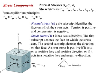
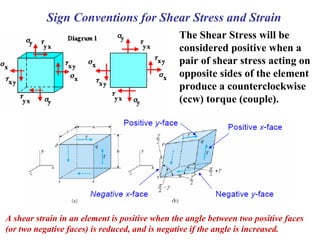
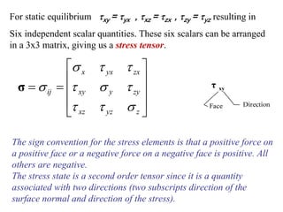
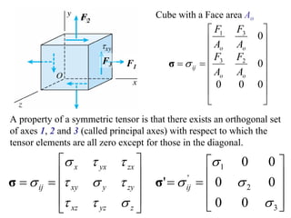
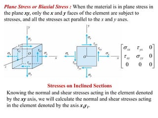
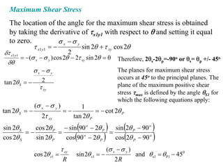
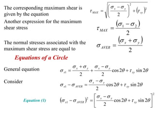
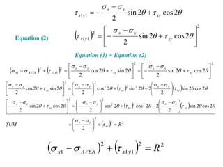
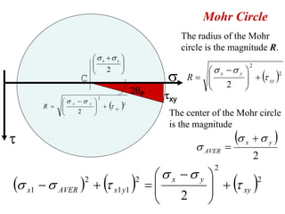
- The document describes a Mechanical Metallurgy course including general information, assessment, textbooks, and tentative dates. - Key topics covered in the course include stress and strain relationships, elasticity theory, plastic deformation, dislocation theory, strengthening mechanisms, and fracture. - Assessment includes partial and final exams, quizzes, attendance, and participation.

1. Mechanical Metallurgy
INME 6016
Pablo G. Caceres‐Valencia
Professor in Materials Science,
B.Sc., Ph.D. (UK)

2. GENERAL INFORMATION
Course Number INME 6016
Course Title Mechanical Metallurgy
Credit Hours 3 (Lecture: 3hours)
Instructor Dr. Pablo G. Caceres‐Valencia
Office Luchetti Building L‐212
Phone Extension 2358
Office Hours Mo and Wed 1:00pm to 5:00pm
e‐mail pcaceres@uprm.edu
pcaceres@me.uprm.edu
Web‐site http://academic.uprm.edu/pcaceres

3. Assessment
The course will be assessed in the following manner:
Partial Exam 30%
Final Exam 30%
Quizzes (3)* 33%
Attendance and Class Participation 7%
(*) A total of three quizzes will be performed.
(**) Class Attendance (after the second absence ‐ 1 point will be deducted for each non‐
authorized absence). The participation in class will be taken into account.
Attendance
Attendance and participation in the lectures are mandatory and will
be considered in the grading. Students should bring calculators,
rulers, pen and pencils to be used during the lectures. Students are
expected to keep up with the assigned reading and be prepared for
the pop‐quizzes or to answer questions on these readings during
lecture.

4. Texbooks
G.E. Dieter; Mechanical Metallurgy; Mc Graw Hill
M.A. Meyers and K.K. Chawla; Mechanical Metallurgy: Principles and
Applications; Prentice‐Hall
I will also post my lecture notes in the web: http://academic.uprm.edu/pcaceres
TENTATIVES DATES
Jan/9‐11 Jan/14‐18 Jan/21‐25
Basic Principles Stress‐Strain Basic Elasticity
Jan/28‐Feb/01 Feb/04‐08 Feb/11‐15
Basic Elasticity Single Crystals Dislocation Theory
Feb/18‐22 Feb/25‐29 Strengthening March/3‐7
Dislocation Theory 1st Exam Mechanisms Strengthening Mechanisms
March/10‐14 Mar/17‐21– Mar/24‐28
Strengthening Mechanisms No Class ‐ Holy Week Fracture
April/1‐4 April/7‐11 Mechanical April /14‐18 Mechanical
Fracture Properties Exam 2 Properties
April/22‐25 – Mechanical Apr/28‐May02‐ Mechanical
Properties Properties

5. Content
•Stress and Strain Relationships for Elastic Behavior
•Elements of the Theory of Elasticity
•Plastic Deformation of Single Crystals
•Dislocation Theory
•Strengthening Mechanisms
•Fracture
•Mechanical Properties

6. The Concept of Stress
Uniaxial tensile stress: A force F is applied perpendicular
to the area (A). Before the application of the force, the
cross section area was AO
F
Engineering stress or nominal stress: Force σ=
divided by the original area. A0
True stress: Force divided by the F
σT =
instantaneous area A
Engineering Strain or Nominal Strain: Change of l − l0 Δl
length divided by the original length ε= =
l0 l0
True Strain: The rate of instantaneous increase in d ⎛ ⎞
the instantaneous gauge length. εT = ∫ = ln ⎜
⎜
⎝
i
o
⎟
⎟
⎠

7. Relationship between engineering and true stress and strain
We will assume that the volume remains Ao o = Ai i
constant.
F F Ao F Ao
σT = = * = *
Ai Ai Ao Ao Ai
Ao Δl + Δl F
= i
= o
= + 1 = (1 + ε ) σT = (1+ ε )
Ai o o o Ao
εT = ∫
d ⎛
= ln ⎜
⎜
i
⎞
⎟
⎟
σ T = σ (1 + ε )
⎝ o ⎠
εT
⎛
= ln ⎜ o + Δ ⎞ ⎛
⎟ ⇒ ln ⎜ o
+
Δ ⎞
⎟ ε T = ln(1 + ε )
⎜ ⎟ ⎜ ⎟
⎝ o ⎠ ⎝ o o ⎠

8. Primary Types of Loading
(a) Tension
(b) Compression
(c) Shear
(d) Torsion
(e) Flexion

9. Hooke’s Law
When strains are small, most of materials are linear elastic.
Young’s modulus
Normal: σ = Ε ε σ
F ⋅ lo
Δl =
Ao ⋅ E
Springs: the spring rate E
F Ao ⋅ E
k= =
Δl lo
ε

10. Torsion Loading resulting from the twist of a shaft.
δθ r ⋅θ
γ θ ,Z = r⋅ ≅ Shear strain
δz l
δθ G ⋅ r ⋅θ
τθ ,z = G ⋅ γ θ ,z = G⋅r ⋅ ≅
δz l
G = Shear Modulus of Elasticity
Twist Moment or Torque
G ⋅θ
T = ∫ r ⋅τ θ , z ⋅ δA = ∫r
2
θ ,z ⋅ δA
A l A
G ⋅θ ⋅ J T ⋅l
T= or θ=
of Inertia A ∫
Area Polar Moment J = r 2 ⋅ δA l G⋅J
Angular spring rate:
T ⋅r T ⋅ ro J ⋅G
Thus: τθ ,z ≅ τ Max ≅ ka = =
T
J J θ l

11. Stress Components Normal Stresses σx, σy, σz
Shear Stresses τxy , τyx , τxz , τzx , τzy , τyz
From equilibrium principles:
τxy = τyx , τxz = τzx , τzy = τyz
Normal stress (σ) : the subscript identifies the
face on which the stress acts. Tension is positive
and compression is negative.
Shear stress (τ) : it has two subscripts. The first
subscript denotes the face on which the stress
acts. The second subscript denotes the direction
on that face. A shear stress is positive if it acts
on a positive face and positive direction or if it
acts in a negative face and negative direction.

12. Sign Conventions for Shear Stress and Strain
The Shear Stress will be
considered positive when a
pair of shear stress acting on
opposite sides of the element
produce a counterclockwise
(ccw) torque (couple).
A shear strain in an element is positive when the angle between two positive faces
(or two negative faces) is reduced, and is negative if the angle is increased.

13. For static equilibrium τxy = τyx , τxz = τzx , τzy = τyz resulting in
Six independent scalar quantities. These six scalars can be arranged
in a 3x3 matrix, giving us a stress tensor.
⎡σ x τ yx τ zx ⎤
⎢ ⎥
σ = σ ij = ⎢τ xy σ y τ zy ⎥
⎢τ xz τ yz σ z ⎥
⎣ ⎦
The sign convention for the stress elements is that a positive force on
a positive face or a negative force on a negative face is positive. All
others are negative.
The stress state is a second order tensor since it is a quantity
associated with two directions (two subscripts direction of the
surface normal and direction of the stress).

14. F2 Cube with a Face area Ao
⎡ F1 F3 ⎤
⎢A 0⎥
Ao
⎢ o ⎥
F3 F1 σ = σ ij = ⎢ F3 F2
0⎥
⎢ Ao Ao ⎥
⎢0 0 0⎥
⎢ ⎥
⎣ ⎦
A property of a symmetric tensor is that there exists an orthogonal set
of axes 1, 2 and 3 (called principal axes) with respect to which the
tensor elements are all zero except for those in the diagonal.
⎡σ x τ yx τ zx ⎤ ⎡σ 1 0 0 ⎤
⎢ ⎥ ⎢0 σ ⎥
σ = σ ij = ⎢τ xy σ y τ zy ⎥ σ ' = σ ij = ⎢
'
2 0⎥
⎢τ xz τ yz σ z ⎥ ⎢ 0 0 σ3⎥
⎣ ⎦
⎣ ⎦

15. Plane Stress or Biaxial Stress : When the material is in plane stress in
the plane xy, only the x and y faces of the element are subject to
stresses, and all the stresses act parallel to the x and y axes.
⎡σ xx τ yx 0⎤
⎢τ σ yy 0⎥
⎢ xy ⎥
⎢ 0
⎣ 0 0⎥
⎦
Stresses on Inclined Sections
Knowing the normal and shear stresses acting in the element denoted
by the xy axis, we will calculate the normal and shear stresses acting
in the element denoted by the axis x1y1.

16. y
y1 x1
θ
x
AO/Cosθ σ
x1
Ao Equilibrium of forces: Acting in x1
θ
σx τx1y1
θ
τxy
τyx AOSinθ/Cosθ
σy
AO Sinθ Sinθ
σ X1 ⋅ = σ X cosθ ⋅ AO + τ XY sinθ ⋅ AO + σY Sinθ ⋅ AO + τYX cosθ ⋅ AO
cosθ Cosθ Cosθ

17. Eliminating Ao , secθ = 1/cosθ
and τxy=τyx
σ X 1 = σ X cos 2 θ + σ Y sin 2 θ + 2τ XY sin θ cos θ
σ Y 1 = σ X sin 2 θ + σ Y cos 2 θ − 2τ XY sin θ cosθ
Acting in y1
τx1y1Aosecθ = − σxAosinθ + τxyAocosθ + σyAotanθcosθ − τyxAotanθsinθ
Eliminating Ao , secθ = 1/cosθ and τxy=τyx
τ x1 y1 = −σ x ⋅ sin θ ⋅ cos θ + σ y ⋅ sin θ ⋅ cos θ + τ xy (cos 2 θ − sin 2 θ )

18. Transformation Equations for Plane Stress
Using the following trigonometric identities:
Cos2θ = ½ (1+ cos 2θ) Sin2θ = ½ (1- cos 2θ) Sin θ cos θ = ½ sin 2θ
σ x +σ y σ x −σ y
σ x1 = + cos 2θ + τ xy sin 2θ
2 2
σ x −σ y
τ x1 y1 = − sin 2θ + τ xy cos 2θ
2
These equations are known as the transformation equations for
plane stress.

19. σ x +σ y σ x −σ y
Special Cases σ x1 = + cos 2θ + τ xy sin 2θ
2 2
σ x −σ y
Case 1: Uniaxial stress τ x1 y1 = − sin 2θ + τ xy cos 2θ
σ y = 0 τ xy = τ yx = 0 2
⎛ 1 + Cos 2θ ⎞
σ x1 = σ x ⋅ ⎜ ⎟
⎝ 2 ⎠
⎛ Sin 2θ ⎞
τ x1, y1 = −σ x ⋅ ⎜ ⎟
⎝ 2 ⎠
Case 2 : Pure Shear
σx =σy = 0
σ x1 = τ xy ⋅ Sin 2θ
τ x1, y1 = τ xy ⋅ Cos 2θ

20. Case 3: Biaxial stress
τ xy = 0
σ x +σ y σ x −σ y
σ x1 = + ⋅ Cos 2θ
2 2
σ x −σ y
τ x1, y1 = − ⋅ Sin 2θ
2

21. Example: An element in plane stress is subjected to stresses
σx=16000psi, σy=6000psi, and τxy=τyx= 4000psi (as shown in figure
below). Determine the stresses acting on an element inclined at an
angle θ=45o (counterclockwise - ccw).
Solution: We will use the following transformation
equations:
σx +σ σ x −σ
σ x1 = + cos 2θ + τ xy sin 2θ
y y
2 2
σ x −σ
τ x1 y 1 = − sin 2θ + τ xy cos 2θ
y
2

22. Numerical substitution
½ (σx + σy) = ½ (16000 + 6000) = 11000psi
½ (σx - σy) = ½ (16000 – 6000) = 5000psi τxy = 4000psi
sin 2θ = sin 90o = 1 cos 2θ = cos 90o = 0 Then
σx1 = 11000psi + 5000psi (0) + 4000psi (1) = 15000psi
τx1y1 = - (5000psi) (1) + (4000psi) (0) = - 5000psi
σx1 + σy1 = σx + σy then σy1 = 16000 + 6000 – 15000 = 7000psi
σ 1 = 17,403 psi
σ 2 = 4,597 psi
τ Max = 6,403 psi

23. Example: A plane stress condition exists at a point on the surface of
a loaded structure such as shown below. Determine the stresses
acting on an element that is oriented at a clockwise (cw) angle of 15o
with respect to the original element.
Solution:
We will use the following transformation equations:
σx +σ σ x −σ
σ x1 = + cos 2θ + τ xy sin 2θ
y y
2 2
σ x −σ
τ x1 y 1 = − sin 2θ + τ xy cos 2θ
y
2

24. Numerical substitution
½ (σx + σy) = ½ (- 46 + 12) = - 17MPa
½ (σx - σy) = ½ (- 46 – 12) = - 29MPa τxy = - 19MPa
sin 2θ = sin (- 30o) = - 0.5 cos 2θ = cos (- 30o) = 0.866 then
σx1 = - 17MPa + ( - 29MPa)(0.8660) + (-19MPa)(- 0.5) = - 32.6MPa
τx1y1 = - (- 29MPa) (- 0.5) + (- 19MPa) (0.8660) = - 31.0MPa
σx1 + σy1 = σx + σy then σy1 = - 46MPa + 12MPa – (- 32.6MPa) = - 1.4MPa

25. Example : A rectangular plate of dimensions 3.0 in x 5.0 in is formed
by welding two triangular plates (see figure). The plate is subjected to
a tensile stress of 600psi in the long direction and a compressive stress
of 250psi in the short direction. Determine the normal stress σw acting
perpendicular to the line or the weld and the shear stress τw acting
parallel to the weld. (Assume σw is positive when it acts in tension and
τw is positive when it acts counterclockwise against the weld).

26. Solution
Biaxial stress weld joint σx = 600psi σy = -250psi τxy = 0
From the figure
tanθ = 3 / 5 θ = arctan(3/5) = arctan(0.6) = 30.96o
We will use the following σ x +σ y σ x −σ y
σ x1 = + cos 2θ + τ xy sin 2θ
transformation equations: 2 2
σ x −σ y
τ x1 y1 = − sin 2θ + τ xy cos 2θ
Numerical substitution 2
½ (σx + σy) = 175psi ½ (σx - σy) = 425psi τxy = 0psi
sin 2θ = sin 61.92o cos 2θ = cos 61.92o
y
25psi -375psi 375psi
Then
σx1 = 375psi τx1y1 = - 375psi Θ=
σx1 + σy1 = σx + σy 30.96o
then σy1 = 600 + (- 250) – 375 = -25psi x

27. Stresses acting on the weld
σw 25psi
τw
375psi
θ
θ = 30.96o
σw = -25psi and τw = 375psi

28. Principal Stresses and Maximum Shear Stresses
The sum of the normal stresses acting on perpendicular faces of
plane stress elements is constant and independent of the angle θ.
σ x +σ y σ x −σ y
σ x1 = + cos 2θ + τ xy sin 2θ
2 2
σ X 1 + σ Y1 = σ X + σ Y
As we change the angle θ there will be maximum and minimum
normal and shear stresses that are needed for design purposes.
The maximum and minimum normal stresses are known as the
principal stresses. These stresses are found by taking the derivative
of σx1 with respect to θ and setting equal to zero.
δσ x1
= −(σ x − σ y ) sin 2θ + 2τ xy cos 2θ = 0
δθ
τ xy
tan 2θ P =
⎛σx −σ y ⎞
⎜
⎜ ⎟
⎟
⎝ 2 ⎠

29. The subscript p indicates that the angle θp defines the orientation of
the principal planes. The angle θp has two values that differ by 90o.
They are known as the principal angles.
For one of these angles σx1 is a maximum principal stress and for
the other a minimum. The principal stresses occur in mutually
perpendicular planes. τ
tan 2θ P = xy
⎛σx −σ y ⎞
⎜
⎜ 2 ⎟ ⎟
⎝ ⎠
τ xy (σ x − σ y )
sin 2θ P = cos2θ P =
R 2R
σ x +σ y σ x −σ y
σ x1 = + cos 2θ + τ xy sin 2θ
2 2
for the maximum stress θ = θ P

30. σ x +σ y σ x −σ y ⎛σ x −σ y ⎞ ⎛τ ⎞ σ x +σ y ⎛ σ x −σ y ⎞ ⎛ 1 ⎞
2
⎟ ⎜ ⎟ + (τ xy )2 ⎜ ⎟
⎛1⎞
σ1 = + ⎜
⎜ ⎟ + τ xy ⎜ xy ⎟ =
⎟ ⎜ ⎟ +⎜
⎜ 2 ⎟ R
2 2 ⎝ 2R ⎠ ⎝ R ⎠ 2 ⎝ ⎠ ⎝ ⎠ ⎝R⎠
σ x +σ y ⎡⎛ σ x − σ y ⎞ 2 ⎤
⎟ + (τ xy ) ⎥
⎛1⎞
σ1 = + ⎜ ⎟ ⎢⎜ ⎜ ⎟
2
2 ⎝ R ⎠ ⎢⎝ 2 ⎠
⎣ ⎥
⎦
⎛ σ x −σ y ⎞ σ x +σ y ⎛ σ x −σ y ⎞
2 2
But ⎜
R= ⎜ ⎟ + (τ xy )2 σ1 = + ⎜
⎜ 2 ⎟ ⎟ + (τ xy )2
⎝ 2 ⎟ ⎠ 2 ⎝ ⎠
⎛σ x +σ y ⎛σ x −σ y
2
⎞ ⎞
⎟ + (τ xy )2
Principal stresses:
σ1 = ⎜
⎜ ⎟+
⎟ ⎜
⎜ ⎟
⎝ 2 ⎠ ⎝ 2 ⎠
⎛σ x +σ y ⎛σ x −σ y
2
⎞ ⎞
σ2 = ⎜
⎜ ⎟−
⎟ ⎜
⎜ ⎟ + (τ xy )2
⎟
⎝ 2 ⎠ ⎝ 2 ⎠
The plus sign gives the algebraically larger principal stress and the
minus sign the algebraically smaller principal stress.

31. Maximum Shear Stress
The location of the angle for the maximum shear stress is obtained
by taking the derivative of τx1y1 with respect to θ and setting it equal
to zero. σ x −σ y
τ x1 y1 = − sin 2θ + τ xy cos 2θ
δτ x1 y1 2
= −(σ x − σ y ) cos 2θ − 2τ xy sin 2θ = 0 Therefore, 2θs-2θp=-90o or θs= θp +/- 45o
δθ
σx −σ y The planes for maximum shear stress
occurs at 45o to the principal planes. The
tan 2θ S = − 2
τ xy plane of the maximum positive shear
stress τmax is defined by the angle θS1 for
which the following equations apply:
(σ x − σ y ) 1
tan 2θ S = − =− = − cot 2θ P
2τ xy tan 2θ P
sin 2θ S
=−
(
cos 2θ P − sin 90 o − 2θ P
= =
)
sin 2θ P − 90 o ( )
cos 2θ S sin 2θ P cos 90 − 2θ P
o
( )
cos 2θ P − 90 o ( )
τ xy (σ x − σ y )
cos 2θ s1 = sin 2θ s1 = − and θ s1 = θ P1 − 450
R 2R

32. ⎛σ x −σ y ⎞
2
The corresponding maximum shear is
τ MAX = ⎜
⎜ ⎟ + (τ xy )2
⎟
given by the equation ⎝ 2 ⎠
Another expression for the maximum (σ 1 − σ 2 )
shear stress τ MAX =
2
(σ x + σ y )
The normal stresses associated with the
maximum shear stress are equal to
σ AVER =
2
Equations of a Circle
σ x +σ y σ x −σ y
General equation σ x1 = + cos 2θ + τ xy sin 2θ
2 2
Consider σ x −σ y
σ x1 − σ AVER = cos 2θ + τ xy sin 2θ
2
⎡σ x − σ y
2
⎤
Equation (1) (σ x1 − σ AVER ) 2
=⎢ cos 2θ + τ xy sin 2θ ⎥
⎣ 2 ⎦

33. σ x −σ y
τ x1 y1 = − sin 2θ + τ xy cos 2θ
2
⎡ σ x −σ y
2
⎤
Equation (2) (τ )
x1 y1
2
= ⎢− sin 2θ + τ xy cos 2θ ⎥
⎣ 2 ⎦
Equation (1) + Equation (2)
⎡σ x − σ y ⎡ σ x −σ y
2 2
⎤ ⎤
(σ x1 − σ AVER )2 + (τ x1 y1 )2 =⎢ cos 2θ + τ xy sin 2θ ⎥ + ⎢− sin 2θ + τ xy cos 2θ ⎥
⎣ 2 ⎦ ⎣ 2 ⎦
⎡σ x − σ y ⎛σ x −σ y ⎛σ −σ y
2 2
⎤ ⎞ ⎞
⎢ cos 2θ + τ xy sin 2θ ⎥ = ⎜
⎜ ⎟ cos 2 2θ + (τ xy )2 sin 2 2θ + 2⎜ x
⎟ ⎜ ⎟(τ xy )sin 2θ cos 2θ
⎟
⎣ 2 ⎦ ⎝ 2 ⎠ ⎝ 2 ⎠
⎡ σ x −σ y ⎛ σ x −σ y ⎛σ −σ y
2 2
⎤ ⎞ ⎞
⎢ − sin 2θ + τ xy cos 2θ ⎥ = ⎜ −
⎜ ⎟ sin 2 2θ + (τ xy )2 cos 2 2θ − 2⎜ x
⎟ ⎜ ⎟(τ xy )sin 2θ cos 2θ
⎟
⎣ 2 ⎦ ⎝ 2 ⎠ ⎝ 2 ⎠
⎛σ x −σ y
2
⎞
SUM =⎜
⎜ ⎟ + (τ xy )2 = R 2
⎟
⎝ 2 ⎠
(σ x1 − σ AVER ) + (τ x1 y1 ) = R 2
2 2

34. Mohr Circle
The radius of the Mohr
circle is the magnitude R.
⎛σ x +σ y ⎞
⎜
⎜ 2 ⎟ ⎟
⎛σ x −σ y
2
⎞
C
⎝ ⎠
σ R= ⎜
⎜ ⎟ + (τ xy )2
⎟
2θP ⎝ 2 ⎠
⎛σ −σ ⎞
2 τxy
R = ⎜
⎜
x y
⎟ +(
⎟ τ xy )
2
⎝ 2 ⎠ The center of the Mohr circle
is the magnitude
τ (σ +σ y )
σ AVER =
x
2
⎛σ x −σ y
2
⎞
(σ x1 − σ AVER ) + (τ x1 y1 ) =⎜ ⎟ + (τ xy )
2 2 2
⎜ ⎟
⎝ 2 ⎠

35. Alternative sign conversion for
shear stresses:
(a) clockwise shear stress,
(b) counterclockwise shear
stress, and
(c) axes for Mohr’s circle.
Note that clockwise shear
stresses are plotted upward and
counterclockwise shear stresses
are plotted downward.
Forms of Mohr’s Circle
a) We can plot the normal stress σx1 positive to the right and the shear
stress τx1y1 positive downwards, i.e. the angle 2θ will be positive
when counterclockwise or
b) We can plot the normal stress σx1 positive to the right and the shear
stress τx1y1 positive upwards, i.e. the angle 2θ will be positive when
clockwise.
Both forms are mathematically correct. We use (a)

36. Two forms of Mohr’s circle:
(a) τx1y1 is positive downward and the angle 2θ
is positive counterclockwise, and
(b) τx1y1 is positive upward and the angle 2θ is
positive clockwise. (Note: The first form is
used here)

37. Construction of Mohr’s circle for plane stress.

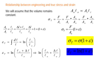
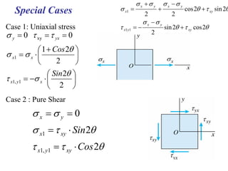
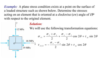
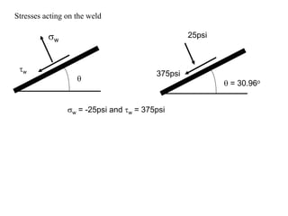
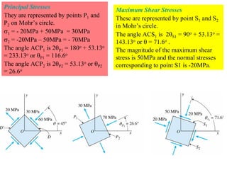
38. Example: At a point on the surface of a pressurized
cylinder, the material is subjected to biaxial stresses
σx = 90MPa and σy = 20MPa as shown in the element
below.
Using the Mohr circle, determine the stresses acting
on an element inclined at an angle θ = 30o (Sketch a
properly oriented element).
Solution (σx = 90MPa, σy = 20MPa and
τxy = 0MPa)
Because the shear stress is zero, these are the
principal stresses.
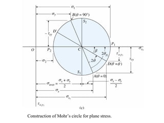
Construction of the Mohr’s circle
The center of the circle is
σaver = ½ (σx + σy) = ½ (90 + 20) = 55MPa
The radius of the circle is
R = SQR[((σx – σy)/2)2 + (τxy)2]
R= (90 – 20)/2 = 35MPa.

39. Stresses on an element inclined at θ = 30o
By inspection of the circle, the coordinates of point D are
σx1 = σaver + R cos 60o = 55MPa + 35MPa (Cos 60o) = 72.5MPa
τx1y1 = - R sin 60o = - 35MPa (Sin 60o) = - 30.3MPa
In a similar manner we can find the stresses represented by point D’, which
correspond to an angle θ = 120o ( 2θ = 240o)
σy1 = σaver - R cos 60o = 55MPa - 35MPa (Cos 60o) = 37.5MPa
τx1y1 = R sin 60o = 35MPa (Sin 60o) = 30.3MPa

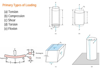
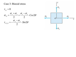
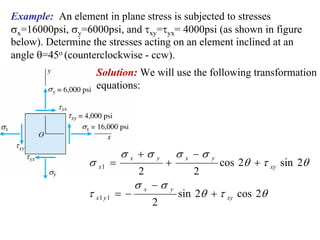
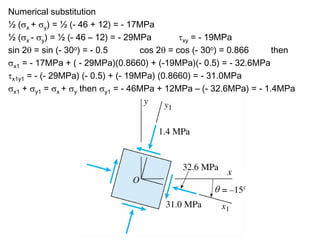
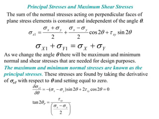
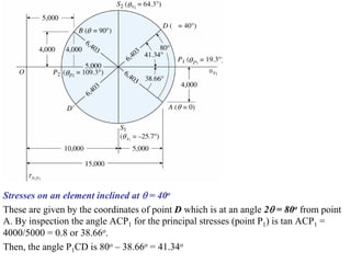
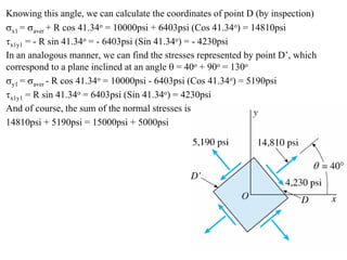
40. Example: An element in plane stress at the
surface of a large machine is subjected to
stresses σx = 15000psi, σy = 5000psi and
τxy = 4000psi, as shown in the figure.
Using the Mohr’s circle determine the following:
a) The stresses acting on an element inclined at
an angle θ = 40o
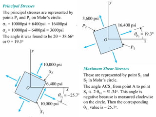
b) The principal stresses and
c) The maximum shear stresses.
Solution
Construction of Mohr’s circle:
Center of the circle (Point C): σaver = ½ (σx + σy) = ½ (15000 + 5000) = 10000psi
Radius of the circle: R = SQR[((σx – σy)/2)2 + (τxy)2]
R = SQR[((15000 – 5000)/2)2 + (4000)2] = 6403psi.
Point A, representing the stresses on the x face of the element (θ = 0o) has the
coordinates σx1 = 15000psi and τx1y1 = 4000psi
Point B, representing the stresses on the y face of the element (θ = 90o) has the
coordinates σy1 = 5000psi and τy1x1 = - 4000psi
The circle is now drawn through points A and B with center C and radius R

41. Stresses on an element inclined at θ = 40o
These are given by the coordinates of point D which is at an angle 2θ = 80o from point
A. By inspection the angle ACP1 for the principal stresses (point P1) is tan ACP1 =
4000/5000 = 0.8 or 38.66o.
Then, the angle P1CD is 80o – 38.66o = 41.34o

42. Knowing this angle, we can calculate the coordinates of point D (by inspection)
σx1 = σaver + R cos 41.34o = 10000psi + 6403psi (Cos 41.34o) = 14810psi
τx1y1 = - R sin 41.34o = - 6403psi (Sin 41.34o) = - 4230psi
In an analogous manner, we can find the stresses represented by point D’, which
correspond to a plane inclined at an angle θ = 40o + 90o = 130o
σy1 = σaver - R cos 41.34o = 10000psi - 6403psi (Cos 41.34o) = 5190psi
τx1y1 = R sin 41.34o = 6403psi (Sin 41.34o) = 4230psi
And of course, the sum of the normal stresses is
14810psi + 5190psi = 15000psi + 5000psi

43. Principal Stresses
The principal stresses are represented by
points P1 and P2 on Mohr’s circle.
σ1 = 10000psi + 6400psi = 16400psi
σ2 = 10000psi – 6400psi = 3600psi
The angle it was found to be 2θ = 38.66o
or θ = 19.3o
Maximum Shear Stresses
These are represented by point S1 and
S2 in Mohr’s circle.
The angle ACS1 from point A to point
S1 is 2 θS1 = 51.34o. This angle is
negative because is measured clockwise
on the circle. Then the corresponding
θS1 value is – 25.7o.

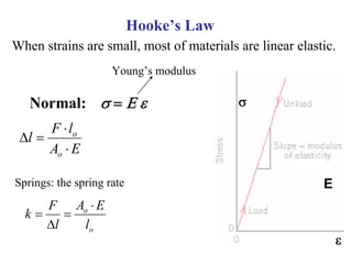
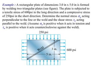
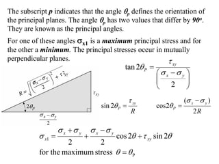
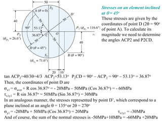
44. Example:At a point on the surface of a
generator shaft the stresses are σx = -50MPa,
σy = 10MPa and τxy = - 40MPa as shown in
the figure. Using Mohr’s circle determine the
following:
(a) Stresses acting on an element inclined at an
angle θ = 45o,
(b) The principal stresses and
(c) The maximum shear stresses
Solution
Construction of Mohr’s circle:
Center of the circle (Point C): σaver = ½ (σx + σy) = ½ ((-50) + 10) = - 20MPa
Radius of the circle: R = SQR[((σx – σy)/2)2 + (τxy)2]
R = SQR[((- 50 – 10)/2)2 + (- 40)2] = 50MPa.
Point A, representing the stresses on the x face of the element (θ = 0o) has the
coordinates σx1 = -50MPa and τx1y1 = - 40MPa
Point B, representing the stresses on the y face of the element (θ = 90o) has the
coordinates σy1 = 10MPa and τy1x1 = 40MPa
The circle is now drawn through points A and B with center C and radius R.

45. Stresses on an element inclined
at θ = 45o
These stresses are given by the
coordinates of point D (2θ = 90o
of point A). To calculate its
magnitude we need to determine
the angles ACP2 and P2CD.
tan ACP2=40/30=4/3 ACP2=53.13o P2CD = 90o – ACP2 = 90o – 53.13o = 36.87o
Then, the coordinates of point D are
σx1 = σaver + R cos 36.87o = - 20MPa – 50MPa (Cos 36.87o) = - 60MPa
τx1y1 = R sin 36.87o = 50MPa (Sin 36.87o) = 30MPa
In an analogous manner, the stresses represented by point D’, which correspond to a
plane inclined at an angle θ = 135o or 2θ = 270o
σy1 = -20MPa + 50MPa (Cos 36.87o) = 20MPa τx1y1 = -30MPa
And of course, the sum of the normal stresses is -50MPa+10MPa = -60MPa +20MPa

46. Principal Stresses Maximum Shear Stresses
They are represented by points P1 and These are represented by point S1 and S2
P2 on Mohr’s circle. in Mohr’s circle.
σ1 = - 20MPa + 50MPa = 30MPa The angle ACS1 is 2θS1 = 90o + 53.13o =
σ2 = -20MPa – 50MPa = - 70MPa 143.13o or θ = 71.6o .
The angle ACP1 is 2θP1 = 180o + 53.13o The magnitude of the maximum shear
= 233.13o or θP1 = 116.6o stress is 50MPa and the normal stresses
The angle ACP2 is 2θP2 = 53.13o or θP2 corresponding to point S1 is -20MPa.
= 26.6o