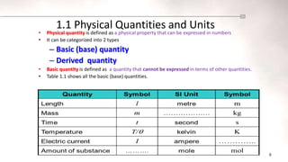
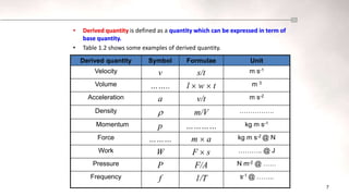
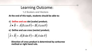
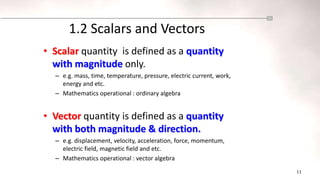
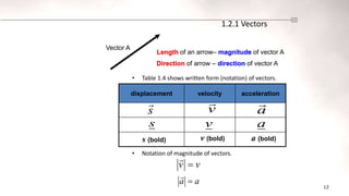
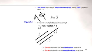
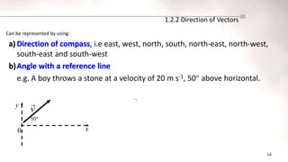
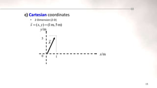
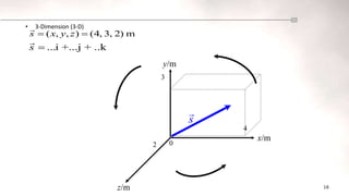
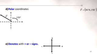
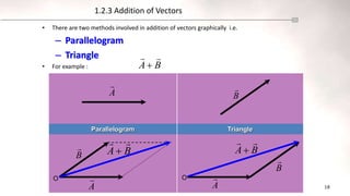
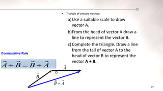
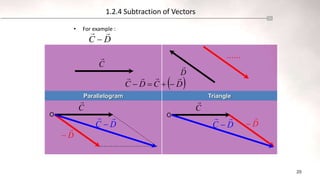
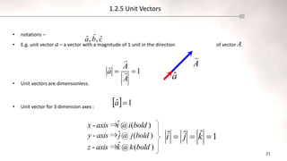
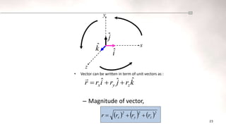
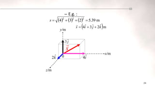
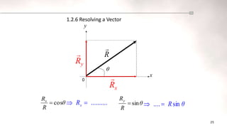
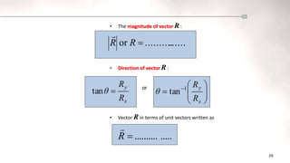
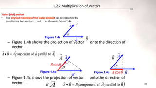
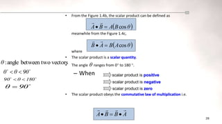
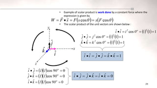
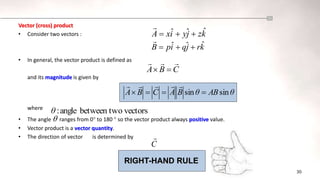
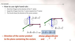
Foundation in engineering and technologyv1

FOUNDATION AND MATRICS SCIENCE
STUDIES
PART 1

1.PHYSICS PART 1
1.PHYSICS
1.1 INTRODUCTION TO PHYSICS
1.2 KINETIC MOTION
1.3 NEWTON LAW

2.MATHEMATICS PART I
1.MATHEMATICS 1
1.1 NUMBER SYSTEMS
1.2 EQUATIONS,INEQUALITIES AND ABSOLUTE
1.3 POLYNOMINALS
1.4 SEQUENCES AND SERIES

PHYSICS CHAPTER 1
1
CHAPTER 1:
Physical quantities and
measurements
(3 Hours)
CHAPTER 1
PHYSI CAL
QUANTI TI ES,
u n i t
AND vect or s

5
At the end of this chapter, students should be able to:
• State basic quantities and their respective SI units: length (m),
time (s), mass (kg), electrical current (A), temperature (K), amount
of substance (mol) and luminosity (cd).
State derived quantities and their respective units and symbols:
velocity (m s-1), acceleration (m s-2), work (J), force (N), pressure
(Pa), energy (J), power (W) and frequency (Hz).
Learning Outcome:
1.1 Physical Quantities and Units (1 hours)
2

6
• Physical quantity is defined as a physical property that can be expressed in numbers
• It can be categorized into 2 types
– Basic (base) quantity
– Derived quantity
• Basic quantity is defined as a quantity that cannot be expressed in terms of other quantities.
• Table 1.1 shows all the basic (base) quantities.
1.1 Physical Quantities and Units

7
• Derived quantity is defined as a quantity which can be expressed in term of
base quantity.
• Table 1.2 shows some examples of derived quantity.
Derived quantity Symbol Formulae Unit
Velocity v s/t m s-1
Volume …….. l  w  t m 3
Acceleration a v/t m s-2
Density  m/V …………….
Momentum p ………… kg m s-1
Force ……… m  a kg m s-2 @ N
Work W F  s ……….. @ J
Pressure P F/A N m-2 @ ……
Frequency f 1/T s-1 @ ……..

8
 It is used for presenting larger and smaller values.
 Table 1.3 shows all the unit prefixes.
1.1.1 Unit Prefixes

9
a)Define scalar and vector quantities,
b)Perform vector addition and subtraction operations
graphically.
c)Resolve vector into two perpendicular components (2-D)
– Components in the x and y axes.
– Components in the unit vectors in Cartesian coordinate.
Learning Outcome:
1.2 Scalars and Vectors

10
At the end of this topic, students should be able to:
d) Define and use dot (scalar) product;
e) Define and use cross (vector) product;
Direction of cross product is determined by corkscrew
method or right hand rule.
Learning Outcome:
   
θ
A
B
θ
B
A
B
A cos
cos 




   
θ
A
B
θ
B
A
B
A sin
sin 





11
• Scalar quantity is defined as a quantity
with magnitude only.
– e.g. mass, time, temperature, pressure, electric current, work,
energy and etc.
– Mathematics operational : ordinary algebra
• Vector quantity is defined as a quantity
with both magnitude & direction.
– e.g. displacement, velocity, acceleration, force, momentum,
electric field, magnetic field and etc.
– Mathematics operational : vector algebra

12
• Table 1.4 shows written form (notation) of vectors.
• Notation of magnitude of vectors.
1.2.1 Vectors
s

Vector A
Length of an arrow– magnitude of vector A
displacement velocity acceleration
v

a

s a
v
v
v 

a
a 

s (bold) v (bold) a (bold)
Direction of arrow – direction of vector A

13
• Two vectors equal if both magnitude and direction are the same. (shown in
figure 1.1)
• If vector A is multiplied by a scalar quantity k
– Then, vector A is
• if k = +ve, the vector is in the same direction as vector A.
• if k = -ve, the vector is in the opposite direction of vector A.
P
 Q

Q
P



Figure 1.1
A
k

A
k

A

A



14
Can be represented by using:
a) Direction of compass, i.e east, west, north, south, north-east, north-west,
south-east and south-west
b)Angle with a reference line
e.g. A boy throws a stone at a velocity of 20 m s-1, 50 above horizontal.
1.2.2 Direction of Vectors
50
v

x
y
0

15
c) Cartesian coordinates
• 2-Dimension (2-D)
m)
5
m,
1
(
)
,
( 
 y
x
s

s

y/m
x/m
5
1
0

16
• 3-Dimension (3-D)
s

2
3
4
m
2)
3,
4,
(
)
,
,
( 
 z
y
x
s

y/m
x/m
z/m
0
...i +...j + ..k
s 

17
d)Polar coordinates
e) Denotes with + or – signs.
 


N,150
30

F
F

150
+
+
-

18
• There are two methods involved in addition of vectors graphically i.e.
– Parallelogram
– Triangle
• For example :
1.2.3 Addition of Vectors
Parallelogram Triangle
B

A

B

A

B
A



O
B
A



B

A

B
A



O

19
• Triangle of vectors method:
a)Use a suitable scale to draw
vector A.
b)From the head of vector A draw a
line to represent the vector B.
c)Complete the triangle. Draw a line
from the tail of vector A to the
head of vector B to represent the
vector A + B.
A
B
B
A







Commutative Rule
B

A

A
B



O

20
• For example :
1.2.4 Subtraction of Vectors
Parallelogram Triangle
D

C

O
D
C



O
......
 
D
C
D
C








C

D


D
C



C

D


D
C




21
• notations –
• E.g. unit vector a – a vector with a magnitude of 1 unit in the direction of vector A.
• Unit vectors are dimensionless.
• Unit vector for 3 dimension axes :
1.2.5 Unit Vectors
A

â
c
b
a ˆ
,
ˆ
,
ˆ
1
ˆ 

A
A
a 

  1
ˆ 
a
)
(
@
ˆ
⇒
- bold
j
j
axis
y 1
ˆ
ˆ
ˆ 

 k
j
i
)
(
@
ˆ
⇒
- bold
i
i
axis
x
)
(
@
ˆ
⇒
- bold
k
k
axis
z

22
• Vectors subtraction can be used
– to determine the velocity of one object relative to another object i.e. to
determine the relative velocity.
– to determine the change in velocity of a moving object.

23
• Vector can be written in term of unit vectors as :
– Magnitude of vector,
x
z
y
k̂
ĵ
iˆ
k
r
j
r
i
r
r z
y
x
ˆ
ˆ
ˆ 



     2
z
2
y
2
x r
r
r
r 



24
– E.g. :
 m
ˆ
2
ˆ
3
ˆ
4 k
j
i
s 



      m
5.39
2
3
4
2
2
2




s
ĵ
3
x/m
y/m
z/m
0
s

i
ˆ
4
k̂
2

25
1.2.6 Resolving a Vector
R

y
R

x
R


0
x
y
θ
R
Rx
cos
 ..........
Rx 
 θ
R
Ry
sin
 θ
Rsin
.... 


26
• The magnitude of vector R :
• Direction of vector R :
• Vector R in terms of unit vectors written as
......
..........
or 
R
R

x
y
R
R
θ 
tan or








 
x
y
R
R
θ 1
tan
.....
..........

R


27
Scalar (dot) product
• The physical meaning of the scalar product can be explained by
considering two vectors and as shown in Figure 1.4a.
– Figure 1.4b shows the projection of vector onto the direction of
vector .
– Figure 1.4c shows the projection of vector onto the direction of
vector .
1.2.7 Multiplication of Vectors
A

B


A

B

A

B

Figure 1.4a

A

B

A

B

θ
B cos
Figure 1.4b

A

B

θ
Acos
Figure 1.4c
 
A
B
A
B
A




to
parallel
of
component


 
B
A
B
B
A




to
parallel
of
component



28
• From the Figure 1.4b, the scalar product can be defined as
meanwhile from the Figure 1.4c,
where
• The scalar product is a scalar quantity.
• The angle  ranges from 0 to 180 .
– When
• The scalar product obeys the commutative law of multiplication i.e.
 
θ
B
A
B
A cos




vectors
o
between tw
angle
:
θ
 
θ
A
B
A
B cos






90
θ
0 
 scalar product is positive


180
θ
0
9 

scalar product is negative

90
θ  scalar product is zero
A
B
B
A








29
• Example of scalar product is work done by a constant force where the
expression is given by
• The scalar product of the unit vectors are shown below :
    1
1
1
cos
ˆ
ˆ 2



 o
2
0
i
i
i
   
θ
F
s
θ
s
F
s
F
W cos
cos 





x
z
y
k̂
ĵ
iˆ
1
ˆ
ˆ
ˆ
ˆ
ˆ
ˆ 




 k
k
j
j
i
i
    1
1
1
cos
ˆ
ˆ 2



 o
2
0
j
j
j
    1
1
1
cos
ˆ
ˆ 2



 o
2
0
k
k
k
   0
9
cos
ˆ
ˆ 

 o
0
1
1
j
i
0
ˆ
ˆ
ˆ
ˆ
ˆ
ˆ 




 k
i
k
j
j
i
   0
9
cos
ˆ
ˆ 

 o
0
1
1
k
i
   0
9
cos
ˆ
ˆ 

 o
0
1
1
k
j

30
Vector (cross) product
• Consider two vectors :
• In general, the vector product is defined as
and its magnitude is given by
where
• The angle  ranges from 0 to 180  so the vector product always positive value.
• Vector product is a vector quantity.
• The direction of vector is determined by
k
r
j
q
i
p
B ˆ
ˆ
ˆ 



k
z
j
y
i
x
A ˆ
ˆ
ˆ 



C
B
A





θ
AB
θ
B
A
C
B
A sin
sin 








vectors
o
between tw
angle
:
θ
RIGHT-HAND RULE
C


31
For example:
– How to use right hand rule :
• Point the 4 fingers to the direction of the 1st vector.
• Swept the 4 fingers from the 1st vector towards the 2nd vector.
• The thumb shows the direction of the vector product.
– Direction of the vector product always perpendicular
to the plane containing the vectors and .
A

C

B
 A

B

C

C
B
A





C
A
B





A
B
B
A






 but  
A
B
B
A








B

)
(C

A


32
THE END…
Next Chapter…
CHAPTER 2 :
Kinematics of Linear Motion

33
CHAPTER 2:
Kinematics of Linear Motion

34
2.0 Kinematics of Linear motion
 is defined as the studies of motion of an objects without considering
the effects that produce the motion.
 There are two types of motion:
 Linear or straight line motion (1-D)
 with constant (uniform) velocity
 with constant (uniform) acceleration, e.g. free fall motion
 Projectile motion (2-D)
 x-component (horizontal)
 y-component (vertical)

35
Learning Outcomes :
• Define and distinguish between
 Distance and displacement
 Speed and velocity
 Instantaneous velocity, average velocity and uniform velocity
 Instantaneous acceleration, average acceleration and uniform acceleration,
• Sketch graphs of displacement-time, velocity-time and acceleration-time.
• Determine the distance travelled, displacement, velocity and acceleration from
appropriate graphs.
2.1 Linear Motion

36
2.1. Linear motion (1-D)
2.1.1. Distance, d
• scalar quantity.
• is defined as the length of actual path between two points.
• For example :
– The length of the path from P to Q is 25 cm.
P
Q

37
 vector quantity.
 is defined as the distance between initial point and final point in a straight line.
 The S.I. unit of displacement is metre (m).
Example 2.1 :
An object P moves 30 m to the east after that 15 m to the south
and finally moves 40 m to west. Determine the displacement of P
relative to the original position.
Solution :
2.1.2 Displacement,
N
E
W
S
O
P


30 m
15 m
10 m 30 m

38
The magnitude of the displacement is given by
and its direction is
2.1.3 Average Speed, v
 is defined as the rate of total distance travelled.
 scalar quantity.
 Equation:
interval
time
travelled
distance
total
speed
Average 
Δt
d
v



39
interval
time
nt
displaceme
of
change

av
v
1
2
1
2
av
t
t
s
s
v



 is a vector quantity.
 The S.I. unit for velocity is m s-1.
Average velocity, vav
 is defined as the rate of change of displacement.
 Equation:
 Its direction is in the same direction of the change in displacement.
2.1.4 Velocity,
Δt
Δs
vav 

40
constant

dt
ds
t
s
0
t
v





limit
Instantaneous velocity, v
 is defined as the rate of change of displacement at the
particular time, t
 Equation:
 An object moves in a uniform velocity when the magnitude and
direction of the velocity remain unchanged.
and the instantaneous velocity equals to the average velocity at
any time.
dt
ds
v 

41
 Therefore
Q
s
t
0
s1
t1
The gradient of the tangent to the curve at point Q
= the instantaneous velocity at time, t = t1
Gradient of s-t graph = velocity

42
interval
time
velocity
of
change

av
a
 vector quantity.
 The S.I. unit for acceleration is m s-2.
Average acceleration, aav
 is defined as the rate of change of velocity.
 Equation:
 Its direction is in the same direction of change in velocity.
 The acceleration of an object is uniform when the magnitude of velocity changes at a
constant rate and along fixed direction.
2.1.5 Acceleration,
1
2
1
2
av
t
t
v
v
a



Δt
Δv
aav 

43
constant

dt
dv
t
v
0
t
a





limit
Instantaneous acceleration, a
 is defined as the rate of change of velocity at the particular time,t.
 Equation:
 An object moves in a uniform acceleration when
and the instantaneous acceleration equals to the average acceleration at
any time.
2
2
dt
s
d
dt
dv
a 


44
 Therefore
v
t
Q
0
v1
t1
The gradient of the tangent to the curve at point Q
= the instantaneous acceleration at time, t = t1
Gradient of v-t graph = acceleration

45
Deceleration, a
 is a negative acceleration.
 The object is slowing down meaning the speed of the object
decreases with time.
Gradient of v-t graph at point C = Negative acceleration
v
t
0
C

46
Displacement against time graph (s-t)
2.1.6 Graphical methods
s
t
0
s
t
0
(a) Uniform velocity (b) The velocity increases with time
Gradient = constant
Gradient increases
with time
(c)
s
t
0
Q
R
P
The direction of
velocity is changing.
Gradient at point R is negative.
Gradient at point Q is zero.
The velocity is zero.

47
 From the equation of instantaneous velocity,
Therefore

48
Velocity versus time graph (v-t)
 The gradient at point A is positive – a > 0(speeding up)
 The gradient at point B is zero – a= 0
 The gradient at point C is negative – a < 0(slowing down)
t1 t2
v
t
0
(a) t2
t1
v
t
0
(b)
t1 t2
v
t
0
(c)
Uniform velocity
Uniform
acceleration
Area under the v-t graph = displacement
B
C
A

49
Learning Outcome :
• Derive and apply equations of motion with uniform
acceleration:
2.2 Uniformly accelerated motion
at
u
v 

2
2
1
at
ut
s 

as
u
v 2
2
2



50
2.2. Uniformly accelerated motion
From the definition of average acceleration,
uniform (constant) acceleration is given by
wherev : final velocity
u : initial velocity
a : uniform (constant) acceleration
t : time
at
u
v 
 (1)
t
u
v
a



51
 From equation (1), the velocity-time graph is shown in Figure 2.4 :
 From the graph,
The displacement after time, s = shaded area under the
graph
= the area of trapezium
 Hence,
velocity
0
v
u
time
t
Figure 2.4
 t
v
u
2
1
s 
 (2)

52
 By substituting eq. (1) into eq. (2) thus
 From eq. (1),
 From eq. (2),
 
 t
at
u
u
s 


2
1
(3)
2
2
1
at
ut
s 

  at
u
v 

 
t
s
u
v
2


multiply
    
at
t
s
u
v
u
v 








2
as
u
v 2
2
2

 (4)

53
 Notes:
 equations (1) – (4) can be used if the motion in a straight
line with constant acceleration.
 For a body moving at constant velocity, ( a = 0) the
equations (1) and (4) become
Therefore the equations (2) and (3) can be written as
u
v 
vt
s  constant velocity

54
Learning Outcome :
• Describe and use equations for freely falling bodies.
– For upward and downward motion, use
a = g = 9.81 m s2
2.3 Freely falling bodies

55
2.3 Freely falling bodies
• is defined as the vertical motion of a body at constant acceleration, g
under gravitational field without air resistance.
• In the earth’s gravitational field, the constant acceleration
– known as acceleration due to gravity or free-fall acceleration or gravitational
acceleration.
– the value is g = 9.81 m s2
– the direction is towards the centre of the earth (downward).
• Note:
– In solving any problem involves freely falling bodies or free fall motion, the
assumption made is ignore the air resistance.

56
 Sign convention:
 Table 2.1 shows the equations of linear motion and freely falling
bodies.
Table 2.1
Linear motion Freely falling bodies
gt
u
v y
y 

y
y
y gs
u
v 2
2
2


2
2
1
gt
t
u
s y
y 

+
- +
-
From the sign convention
thus,

57
THE END…
Next Chapter…
CHAPTER 3 :
Newton's Law & Its application

CHAPTER 3:
NEWTON’S LAW OF
MOTION AND ITS
APPLICATIONS

59
Learning Outcome:
 Identify the forces acting on a body in different situations:
◦ Weight
◦ Tension
◦ Normal Force
◦ Friction
 Draw free body diagram.
 Determine the resultant force.
3.1 INTRODUCTION

60
• is defined as something capable of changing state of motion or size or dimension
of a body.
• There are 4 types of fundamental forces in nature:
a) Gravitational forces
b) Electromagnetive forces
c) Strong nucleur forces
d) weak nucleur forces
3.1.1 Basic of Forces & Free body diagram
• Since force has magnitude and direction, it is a vector quantity
• If several forces acts simultaneously on the same object, it is
the net force that determines the motion of the object.
• The net force is the vector sum of all the forces acting on the object
and it is often called resultant force.
The magnitude of a force can
be measured using a spring
scale.

62
• It always directed toward the centre of the earth or in
the same direction of acceleration due to gravity, g.
g
m
W



Weight (Force),
• Weight is defined as the force with which a body is attracted
towards the center of the earth.
• It is dependant on where it is measured, because the
value of g varies at different localities on the earth’s
surface.
• It is a vector quantity.
Equation:
• The S.I. unit is kg m s-2 or Newton (N).
W


63
W
All the W pointing downward as shown in figure 3.1.1 above
Figure 3.1.1

64
Tension,
• Tension is the magnitude of the pulling force that is directed
away from the object and attempts to stretch & elongate
the object. (figure 3.1.2)
• Measured in Newton and is always parallel to the string on
which it applies.
Single string system:
T
T
T
m1 m1 m1
ϴ
Figure 3.1.2

65
T T
T
T
m1
Single string system (smooth pulley)
Multiple string system
m1 m2
T2
T2 T3 T3
The tension T acts for the whole
one string but it will be different
if it acts on different masses, T1
and T2 as shown in fig 3.1.3 and
Fig 3.1.4
Fig 3.1.3
Fig 3.1.4
T1

66
m4
m1
m2
m3
T3
T1 T1
T1
T1
T2 T2
T2
T2
T3 T3
T3
Multiple string system (inclined plane)
The are three different tension T1, T2 and T3
acts on different masses of m1, m2 and m3
as shown in fig 3.1.5.
Fig 3.1.5

67
N1
N2
N3
m1
m2
m3
Surface 1
Surface 2
Surface 3
Normal Force (Reaction Force), N or R
is the contact force component , which is perpendicular to the surface
of contact and exerted on an object by preventing the object from
penetrating the surface. (fig 3.1.6)
Fig 3.1.6

Frictional force,
68
N
f 

force
frictional
:
f
friction
of
t
coefficien
:
μ
where
• is defined as a force that resists the motion of one surface
relative to another with which it is in contact.
• is independent of the area of contact between the two surfaces
• is directly proportional to the reaction force.
f


69
Figure 3.1.7
N
fs
W
F
N
W
F
N
W
F
fs = max fk
Block at rest Block about to slide Block is sliding
There are three different stages of friction acts on a block
which are going to slide as shown in figure 3.1.7.

Free Body Diagram
70
• is defined as a diagram showing the chosen body by
itself, with vectors drawn to show the magnitude &
directions of all the forces applied to the body by the other
bodies that interact with it.
• A single point may represent the object.
Example : Sketch free body diagrams for each case
Case 1 : Horizontal surface
a) An object lies at rest on a flat horizontal surface
m

F
b) A box is pulled along a rough horizontal surface by a
horizontal force, F
m
a
Case 2 : Inclined Plane
A box is pulled up along a rough inclined plane by a force, F
m

72
Case 3 : Hanging object
An object is hang by using a light string
m
m

73
Case 4 : Pulley
m1
m2
m2
m1

Learning Outcome:
 State Newton’s First Law
 Define mass as a measure of inertia.
 Define the equilibrium of a particle.
 Apply Newton’s First Law in equilibrium of forces.
 State and apply Newton’s Second Law.
 State and apply Newton’s Third Law.
74
3.2 Newton's Law of Motion

3.2 Newton’s laws of motion
states “an object at rest will remain at rest, or continues
to move with uniform velocity in a straight line unless it
is acted upon by a external forces”
75
Inertia
is defined as the tendency of an object to resist any change
in its state of rest or motion.
is a scalar quantity.
Newton’s first law of motion
The first law gives the idea of inertia.
0


 F
Fnett

• Figures 3.2 show the example of real experience of inertia.
76
Figure 3.2
Equilibrium of object / particle
The resultant of forces is zero. (Translational equilibrium)
Equilibrium of object / particle occurs when the net force
exerted on it is zero.
Newton’s 1st law of motion
0

F

interval
time
:
dt
77
its can be represented by
where force
resultant
:
F

State and apply Newton’s Second Law.
states “the rate of change of linear momentum of a moving body
is proportional to the resultant force and is in the same direction
as the force acting on it”
dp : Change in momentum
dt
dp
F 


If the forces act on an object and the object moving at
uniform acceleration (not at rest or not in the equilibrium)
hence
78
Newton’s 2nd law of motion restates that “The acceleration of an
object is directly proportional to the nett force acting on it and
inversely proportional to its mass”.
One newton(1 N) is defined as the amount of nett force that
gives an acceleration of one metre per second squared to a
body with a mass of one kilogramme. 1 N = 1 kg m s-2
is a nett force or effective force or resultant force.
The force which causes the motion of an object.
F

m
F
a

 

ma
F
Fnett 




Newton’s third law of motion
79
For example :
When the student push on the wall it will push back with
the same force. (refer to Figure 3.2.1)
A (hand)
B (wall)
Figure 3.2.1
is a force by the hand on the wall (action)
Where
is a force by the wall on the hand (reaction)
states “every action force has a reaction force that is equal in
magnitude but opposite in direction”.
BA
AB F
F




AB
F

BA
F


80
A rocket moves forward as a result of the push exerted on it
by the exhaust gases which the rocket has pushed out.
Figure 3.2.2
Force by the book on the table (action)
Force by the table on the book (reaction)
When a book is placed on the table. (refer to Figure 3.2.2)
If a car is accelerating forward, it is because its tyres are pushing
backward on the road and the road is pushing forward on the tyres.
In all cases when two bodies interact, the action and reaction
forces act on different bodies.

81
The motion of an elevator can give rise to the sensation
of being heavier or lighter.
Apparent weight
The force exerted on our feet by the floor of the elevator.
If this force is greater than our weight, we felt heavier, if
less than our weight , we felt lighter.

Case 1 : Motion of a lift
 Consider a person standing inside a lift as shown in
Figures 3.2.7a, 3.2.7b and 3.2.7c.
a. Lift moving upward at a uniform velocity
82
Since the lift moving at a
uniform velocity, thus
Therefore
Figure 3.2.7a mg
N
mg
N
Fy





0
0
N

b. Lift moving upwards at a constant acceleration, a
83
By applying the newton’s 2nd
law of motion, thus
Figure 3.2.7b
)
( g
a
m
N
ma
mg
N
ma
F y
y







c. Lift moving downwards at a constant acceleration, a
84
By applying the newton’s 2nd
law of motion, thus
Figure 3.2.7c
 Caution : N is also known as apparent weight and
W is true weight.
)
( a
g
m
N
ma
N
mg
ma
F y
y






mg
W 

Case 2 : An object on Horizontal surface
 Consider a box of mass m is pulled along a horizontal
surface by a horizontal force, F as shown in Figure 3.2.8
85
Figure 3.2.8
 
 ma
F
F nett
x ma
f
F 

  0
y
F mg
N 
x-component :
y-component :
mg
N

prepared by NASS
CHAPTER 1&2
• REAL AND COMPLEX NUMBERS
• INDICES, SURD & LOGARITHM

prepared by NASS
 Define real numbers, all the subsets of real numbers, complex
numbers, indices, surds & logarithm.
 Represent the relationship of number sets in a real number system
diagrammatically.
 Understand open, closed and half-open intervals and their
representations on the number line.
 Simplify union, and intersection of two or more intervals with the
aid of the number line.
 Perform operations on complex number.
 Simplify indices, surds & logarithm.

prepared by NASS
REAL LINE
0 2.5 10
-9 -1
To the right, getting bigger
To the left, getting smaller

prepared by NASS
Intervals of Real Numbers
Can be illustrated using:
Set Notation
Interval/Bracket Notation
Real number line
S
R
I

prepared by NASS
Summary of Real Numbers Interval
Set Notation Interval Notation Real Number Line Notation
 
b
x
a
x 

:
 
b
x
a
x 

:
 
a
x
x 
:
 
a
x
x 
:
 
a
x
x 
:
 
a
x
x 
:
 

,
a
 
a
,


 
a
,


 
b
a,
 
b
a,
 

,
a
a
a
a
a
a b
a b

Example:
Write the following set of real numbers using a real number line and interval notation.
1. The set of real numbers less than 10. ;
2. The set of real numbers greater than or equal to 5. ;
3. The set of real numbers greater than -5 but less than or equal to 9.
;
4. The set of real numbers between 7 and 20. ;
prepared by NASS
10
 
10
,


5
 

,
5
5 9
 
9
,
5
7
20
)
20
,
7
(

prepared by NASS
Combining Intervals
Union : the set of real numbers that belong to either one or both of
the intervals.
A B = { x | x A or x B }
Intersection : the set of real numbers that belong to both of the
intervals.
A B = { x | x A and x B }
  




prepared by NASS
Example: Write each union/intersection as a single interval.
   
9
,
3
5
,
1 
   
9
,
3
5
,
1 
   


 ,
0
3
,
4
   


 ,
0
3
,
4
5 9
1 3
 
9
,
1
5 9
1 3
 
5
,
3
3
-4 0
 

 ,
4
3
-4 0
 
3
,
0

Is any number of the form ,which cannot be written as a fraction of two
integers is called surd.
Properties of Surds:
b
 
a
a
a
b
c
a
b
c
b
a
b
a
b
a
ab
b
a








4)
3)
2)
1)

chapter 1 96
Conjugate Surds
a b a b
  
RATIONALIZING DENOMINATORS
Problem arise when algebraic fraction involving surds in the denominator.
Solution:
1) Eliminate the surd from denominator by multiplying the numerator and
denominator by the conjugate of the denominator.

Is a set of number in form,
Where and are real numbers and . A complex number is
generally denoted by,
prepared by NASS
bi
a 
Real part, Re(z) Imaginary part, Im(z)
a b 1


i
bi
a
z 


prepared by NASS
Equality of complex numbers .
Conjugate of complex numbers .
bi
a
z 
 bi
a
z 

is the complex number obtained by changing the sign of the
imaginary part of .
z

prepared by NASS
• Addition/Subtraction
• Multiplication
• Division
       i
d
b
c
a
di
c
bi
a 






      i
bc
ad
bd
ac
di
c
bi
a 





 
2
2
2
2
d
c
i
ad
bc
d
c
bd
ac
di
c
bi
a








Algebraic Operations of Complex
Numbers

prepared by NASS
If a is a real number and n is a positive integers,
then
Where, a = base
n = index
a
a
a
a
an




 ...
n times

1)
2)
3)
4)
5)
prepared by NASS
Rules/Law of Indices
n
m
n
m
a
a
a 

  mn
n
m
a
a 
n
m
n
m
a
a
a 

  0
, 
 b
b
a
ab m
m
m
0
, 







b
b
a
b
a
m
m
m
0
;
1



a
a
a n
n
6)
0
a
;
1
a0


7)
8)
0
a
;
a
a n m
n
m



prepared by NASS
Definition: The logarithm of any number of a
given base is equal to the power to
which the base should be raised to get the
given number.
From indices, a, x and n are related such that
Then, x is said to be the logarithm of n wrt the
base a.
n
ax

log𝑎 𝑛 = 𝑥

1) 6)
2) 7)
3)
4)
5)
prepared by NASS
Rules/Law of Logarithm
n
log
m
log
)
mn
(
log a
a
a 

n
log
m
log
n
m
log a
a
a 







m
log
n
m
log a
n
a 
a
log
m
log
m
log
b
b
a 
0
1
loga 
1
a
loga 
n
a n
a
log


MATHEMATICS 1 SEQUENCE AND SERIES
• Centre for Foundation Studies

Sequence and Series
•Sequence and
series
•Arithmetic
progression
•Geometric
progression
•Binomial expansion

Sequence and series
•Defn of sequence
•Types of sequence
•General term of
sequence
•Defn of series
•Types of series

Sequence
Definition
• Sequence- A set of order numbers.
• Terms – the numbers which form
the sequence, denoted by T1,
T2,T3,…….
Type
• Finite – containing a finite number of
terms.
•Infinite – have an unlimited number of
terms. General Term

General term of a sequence
• The nth term of the sequence of even
numbers
Tn =2n
• The nth term of the sequence of odd
numbers
Tn =2n-1
• The nth term
of
1 1 1 1
, , ,
3 5 9 17
1
,..... is given by Tn  n
2 1

Series
n
Definition
• The sum of the terms in a
sequence.
• Finite series
Ti  T1 T2 T3 ....Tn  Sn
i1
• Infinite series
 T1  T2  T3  ...  S

 Ti
i1

Arithmetic Progression
• Arithmetic progression can be either
arithmetic sequence or arithmetic
series.
• Arithmetic sequence
- A sequence whose consecutive terms
have a
constant difference.
- a, a+d, a+2d,…….,a+(n-1)d.
-The first term- ‘a’
-Fixed difference – ‘d’ also known as
common difference. Can be positive or

Arithmetic series
Definition
• The sum of arithmetic
sequence
2 2
n n
S 
n
2a  (n 1)d  or S 
n
(a  l)
l  a  (n 1)d
• Arithmetic mean for two numbers
- If a,b,c is an arithmetic sequence, then
b is arithmetic mean of a and c.
b 
a  c
2

Arithmetic series
If a and b are two numbers
and A1,A2,A3,…..,An are
arithmetic means between
a and b, then a,
A1,A2,A3,…..,An ,b are in
arithmeticsequence.

Geometric progression
sequenc
e
n
where r is common ratio
a is the first term
Geometric series – The sum of a
geometric
Geometric sequence – A sequence in
which the ratio of any two consecutive
terms is a constant. . T  arn1
a(1rn
)
When r  1, use Sn 
or
When r  1, use Sn 
1  r
a(rn
1)
r 1

Geometric mean
• If a,b,c is a geometric sequence, then
the geometric mean of a and c is b,
where
b2
 ac
b   ac
• Sum to infinity of the geometric series
where r  1
1  r
a

S 

Application of arithmetic and geometric series
• An engineer has an annual salary of RM24,000
in his first year. If he gets a raise of RM3,000
each year, what will his salary be in his tenth
year? What is the total salary earned for 10
years of work?
• CFS launched a reading campaign for students
on the first day of July. Students are asked to
read 8 pages of a novel on the first day and
every day thereafter increase their daily
reading by one page. If Saddam follows this
suggestion, how many pages of the novel will

Application of arithmetic and geometric series
• Aida deposits RM5,000 into a bank that
pays an interest rate of 5% per annum. If
she does not withdraw or deposit any
money into his account, find the total
savings after 10 years.
• Each year the price of a car depreciates
by 9% of the value at the beginning of the
year. If the original price of the car was
RM60,000. Find the price of the car after
10 years.

Binomial expansion
Denoted
by
Binomial
theorem
 a  b  n
 
abn

n
an
b0

n
an1
b1
..............
n
a0
bn
0 1 
where
n!
k!(nk)!
n
n
ab  a b
nk k
k
n
n
n

 k
 
k0  
     
 


General term
• If n is a negative integer or a rational number, then
•1 xn
1
n
x
nn1x2

nn1n2x3
......
• 1 2! 3!
• provided -1 x 1 or x  1
General term-The (r+1)th term of
the expansion of (a+b)n is denoted
by Tr+1 .
T r1

n
anr
br
 r
 

• Perform addition, subtraction, multiplication and division of
polynomials.
• Use the remainder and factor theorems in problem solving.
• Find the roots and zeros of a polynomial.
• Perform partial fraction decomposition when the denominators are
in the form of:
– A linear factor.
– A repeated linear factor.
– A quadratic factor
At the end of this chapter, student should be able to:

Polynomials
1 2
1 2 1 0
0
Polynomial function ( ) is
( ) .....
where,
- leading coefficient, 0
- degree of the polynomial & positive integer
- constant term
n n
n n
n n
P x
P x a x a x a x a x a
a a
n
a


     


Steps to be taken:
S1 Divide the 1st term of numerator, P(x) by the 1st term of denominator,
D(x) answer, Q(x).
S2.Multiply the denominator, D(x) by the answer and put below
numerator.
S3 Subtract to create a new polynomial.
S4.Repeat S1 using the new polynomial until the degree of new
polynomial is less than denominator.

Example
2
3 2
Multiply:(2 3)(3 2 3)
4 5 2
Use long division to find
2
x x x
x x x
x
  
  


Remainder Theorem
Example:
refer example 1 and 2 in textbook page 234.
Note: If a polynomial is divided by a quadratic expression, then
the remainder, R = Ax + B. Where A and B are constant to be
determined.
If R is the remainder after dividing
the polynomial P(x) at (x-a), then
P(a)=R

Factor Theorem
For a polynomial P(x) and a constant a,
iff P(a) = 0, then (x - a) is a factor of
P(x).

Zeros of Polynomials
The zeros of the polynomial can be obtained
when P(x) is completely factorised and then
solved for zero.
Therefore a, b and c are zeros of the
polynomial
P(x).
If ( ) ( )( )( ),
then ( ) 0, ( ) 0 and ( ) 0.
P x x a x b x c
P a P b P c
   
  

3 2
3 2
If ( ) ( )( )( ),
then , and are called the roots of
the polynomial equation ( ) 0
Example:
( ) 2 5 6
( ) ( 1)( 2)( 3)
then the zeros are 1,-2 and 3.
1 is a root of ( ) 2 5
P x x a x b x c
x a b c
P x
P x x x x
P x x x x
x P x x x
   


   
   
    6
since (1) 0.
x
P



Partial fraction
If the degree of P(x) is less than that of D(x), then
is called a proper fraction.
Only a proper rational expression can be expressed as
partial fractions.
( )
( )
P x
D x
partial fraction
decomposition
Non-
repeated
Linear
Repeated
linear
Non-
repeated
quadratic
Repeated
quadratic

Partial fractions decomposition
Case 1:Denominator consists of non-repeated linear factors.
 Contain an expression of the form for each
non-repeated linear factor (ax+b) in the denominator.
A
ax b


Case 2: Denominator consists repeated linear
factors.
 Contain an expression of the form
for each repeated linear factor of multiplicity n.
   
2
1
2
..... n
n
A A
A
ax b ax b ax b
  
  

Case 3: Denominator consists of non-repeated quadratic
factors.
 If a non-reducible factor, occur
in the denominator, then the partial fraction
corresponding to this factor is
2
ax bx c
 
2
Ax B
ax bx c

 

Case 4: Denominator consists of repeated
quadratic factors.
 If the factor is repeated twice
in the denominator, then the form of the
partial fractions corresponding to this would
be
2
ax bx c
 
 
2
2 2
Ax B Cx D
ax bx c ax bx c
 

   

Improper rational expression
Improper rational expression is when the
degree
of P(x) greater than D(x).
S1: long division
S2: partial fraction
reduce the
improper rational
expression to proper
rational expression

Foundation in engineering and technologyv1

More Related Content

What's hot

Similar to Foundation in engineering and technologyv1

More from Reema

Recently uploaded

Foundation in engineering and technologyv1