The document outlines forecasting methods in operations management used by Tupperware, detailing various types of forecasts (short, medium, long-range) and their relevance to business decisions such as sales, production, and staffing. It discusses different forecasting methodologies including qualitative methods like the jury of executive opinion and quantitative approaches such as moving averages and exponential smoothing. The importance of understanding product life cycles and the limitations of forecasting accuracy are also highlighted.

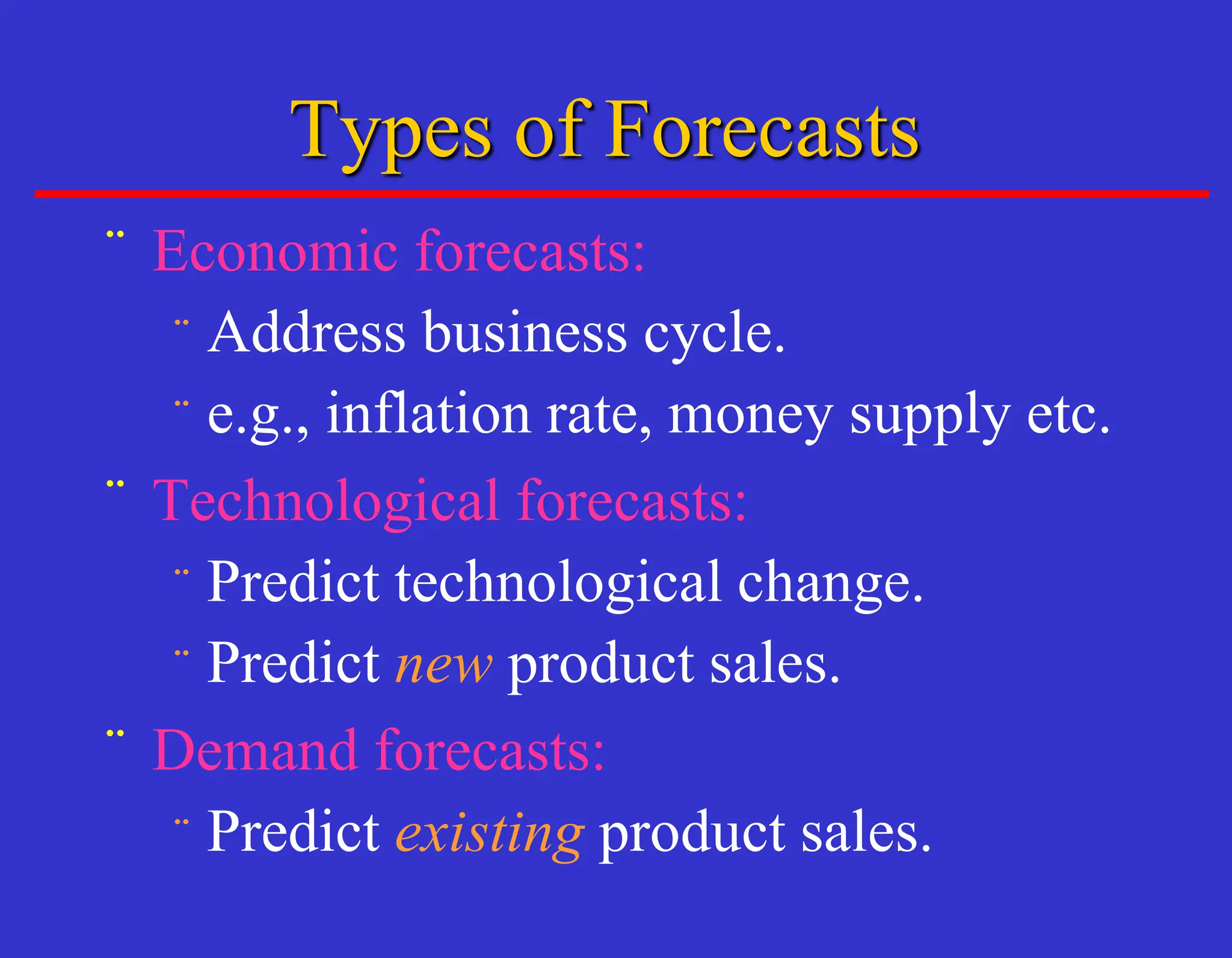
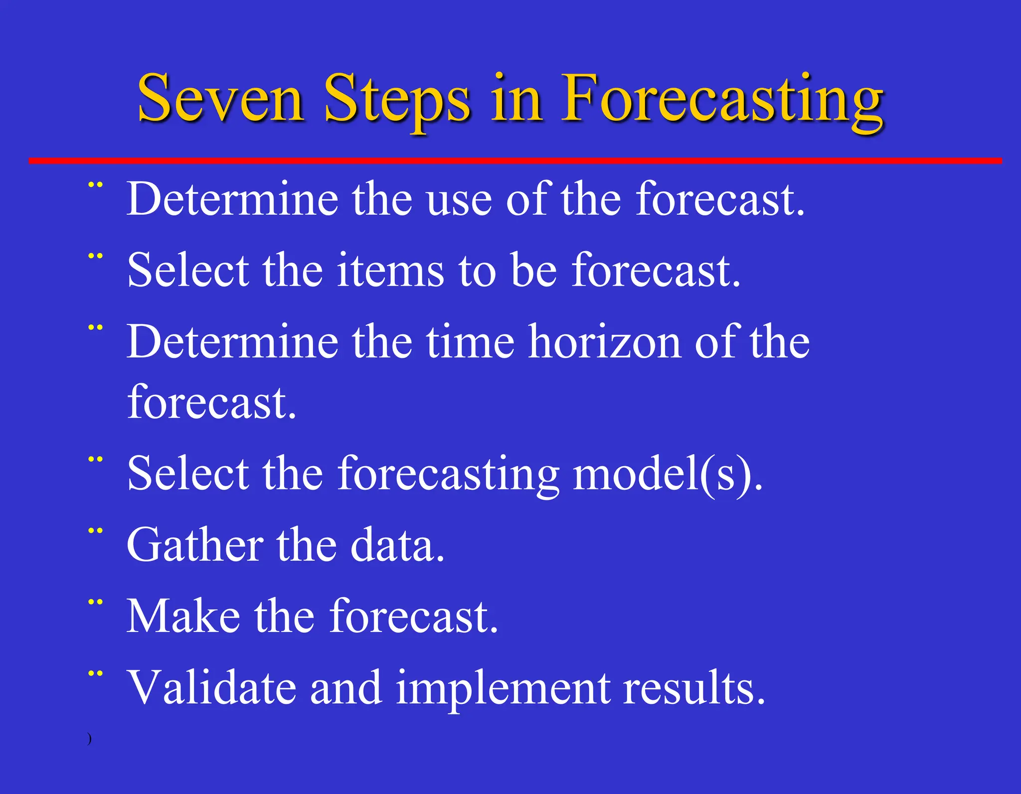
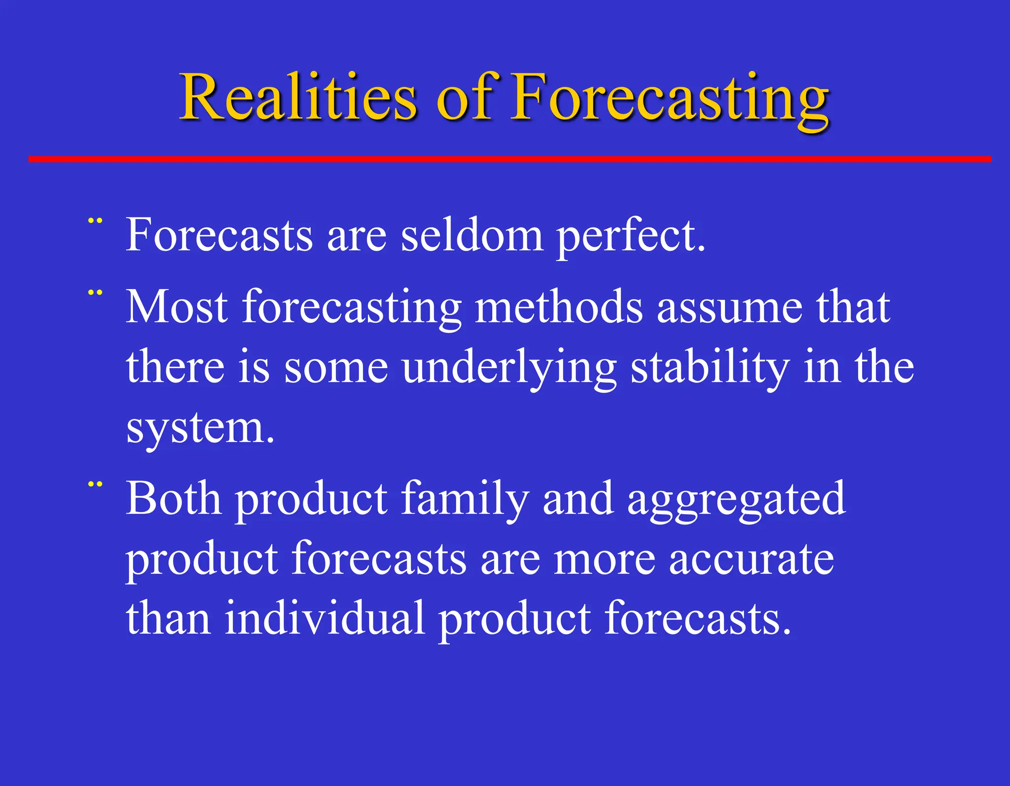
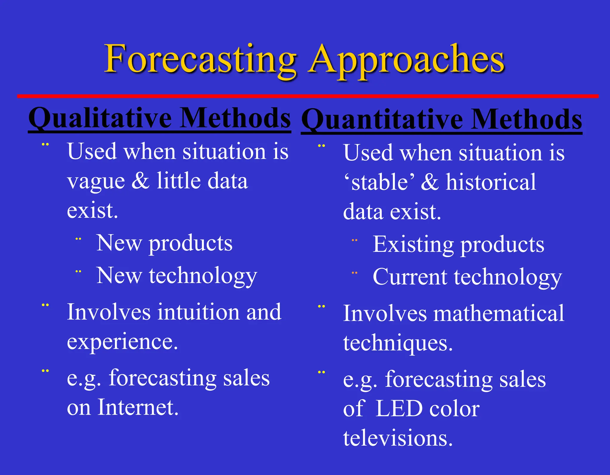
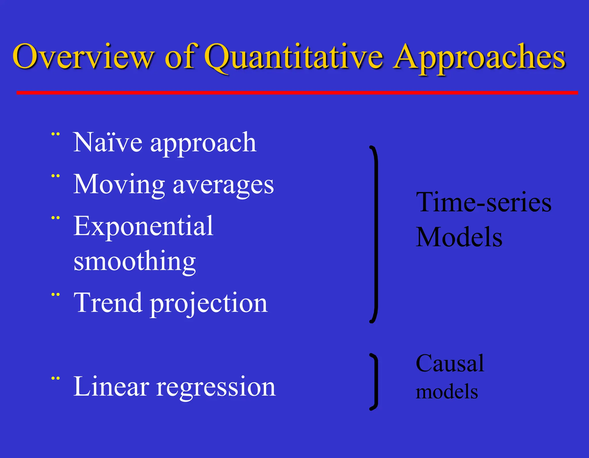
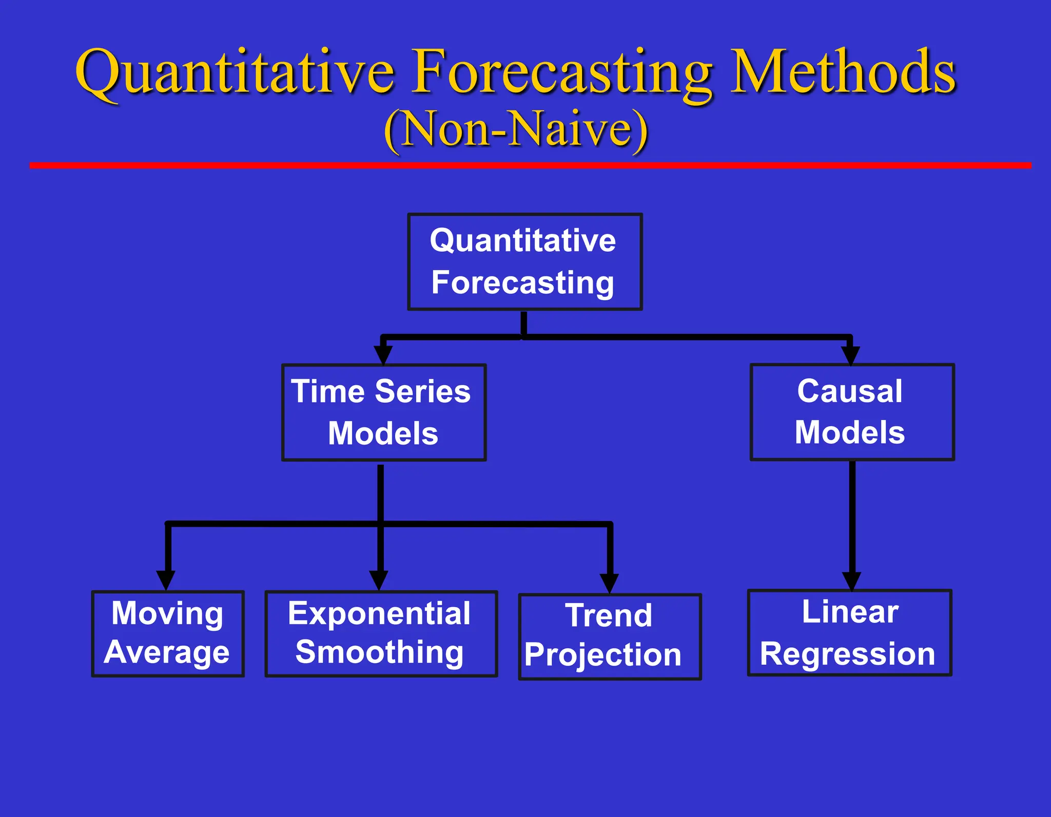
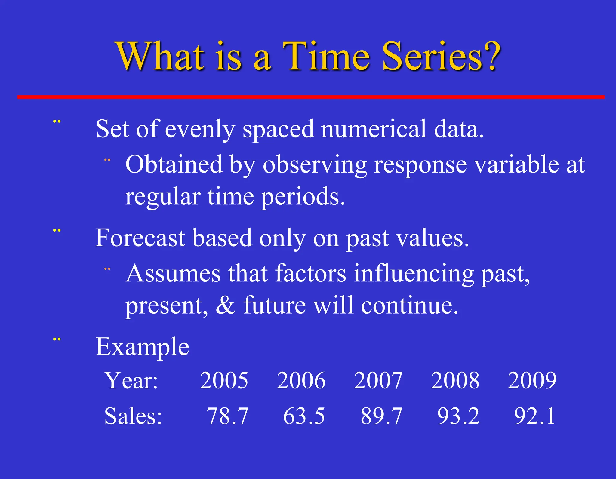
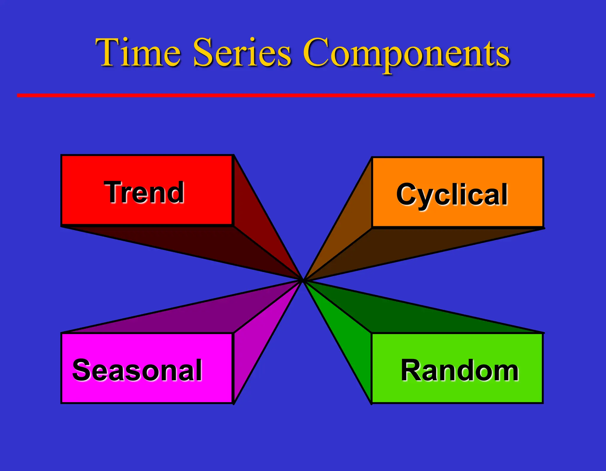
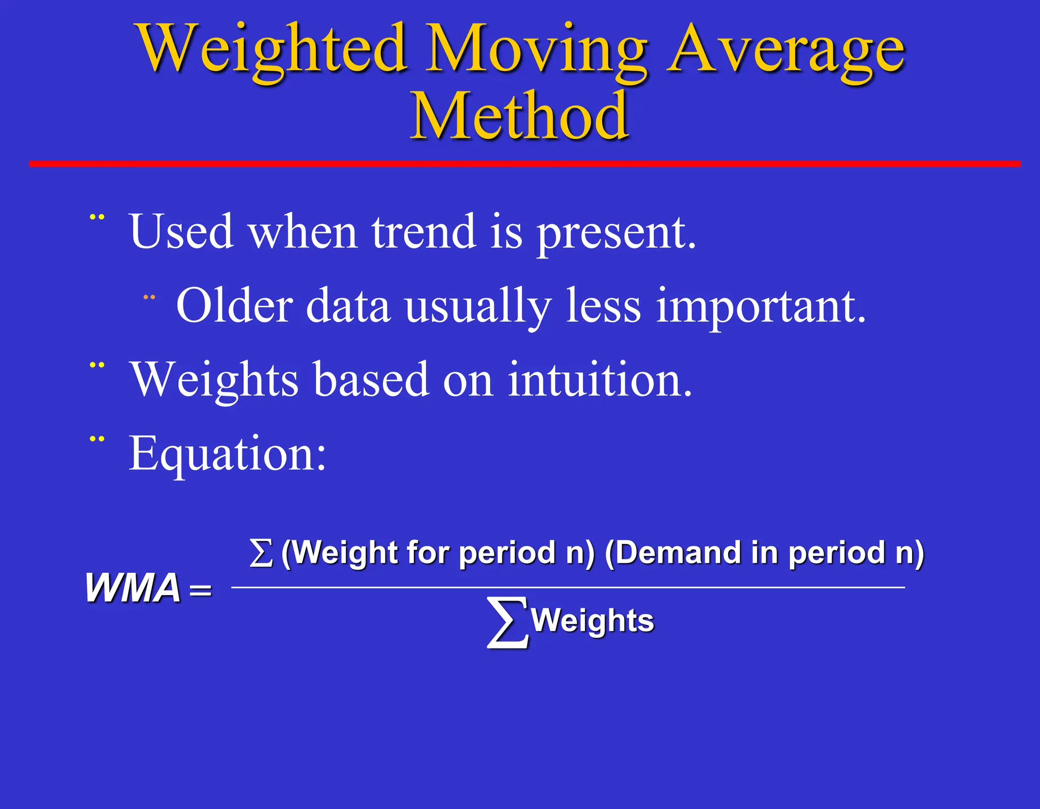
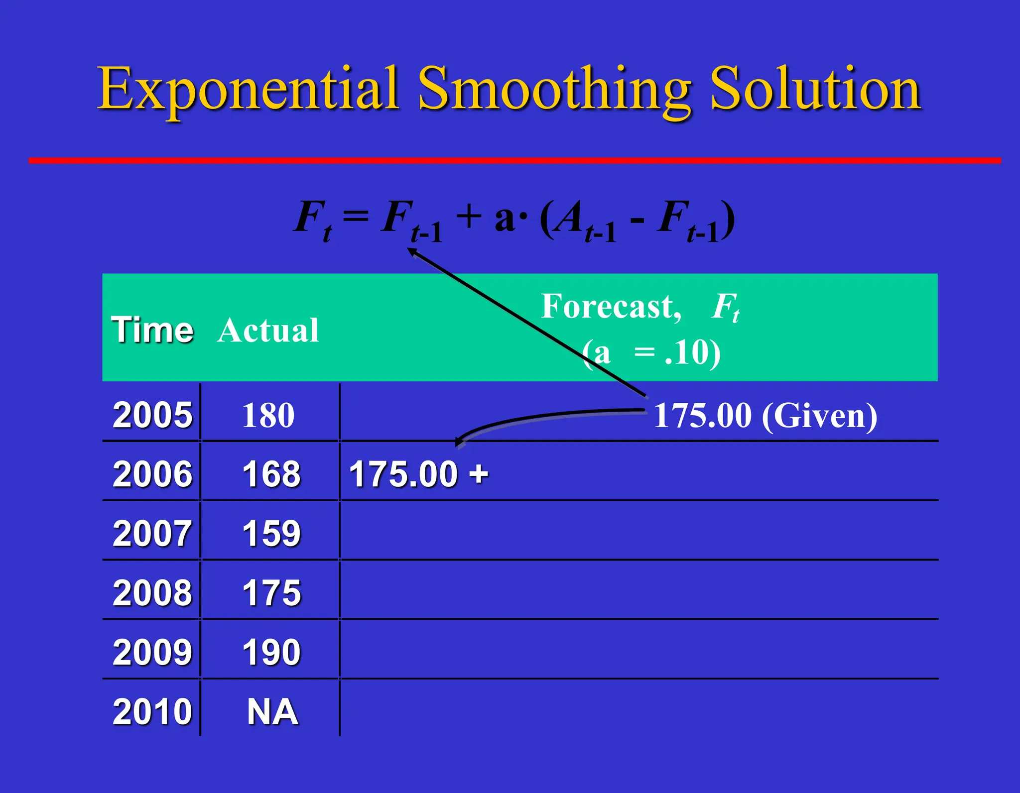
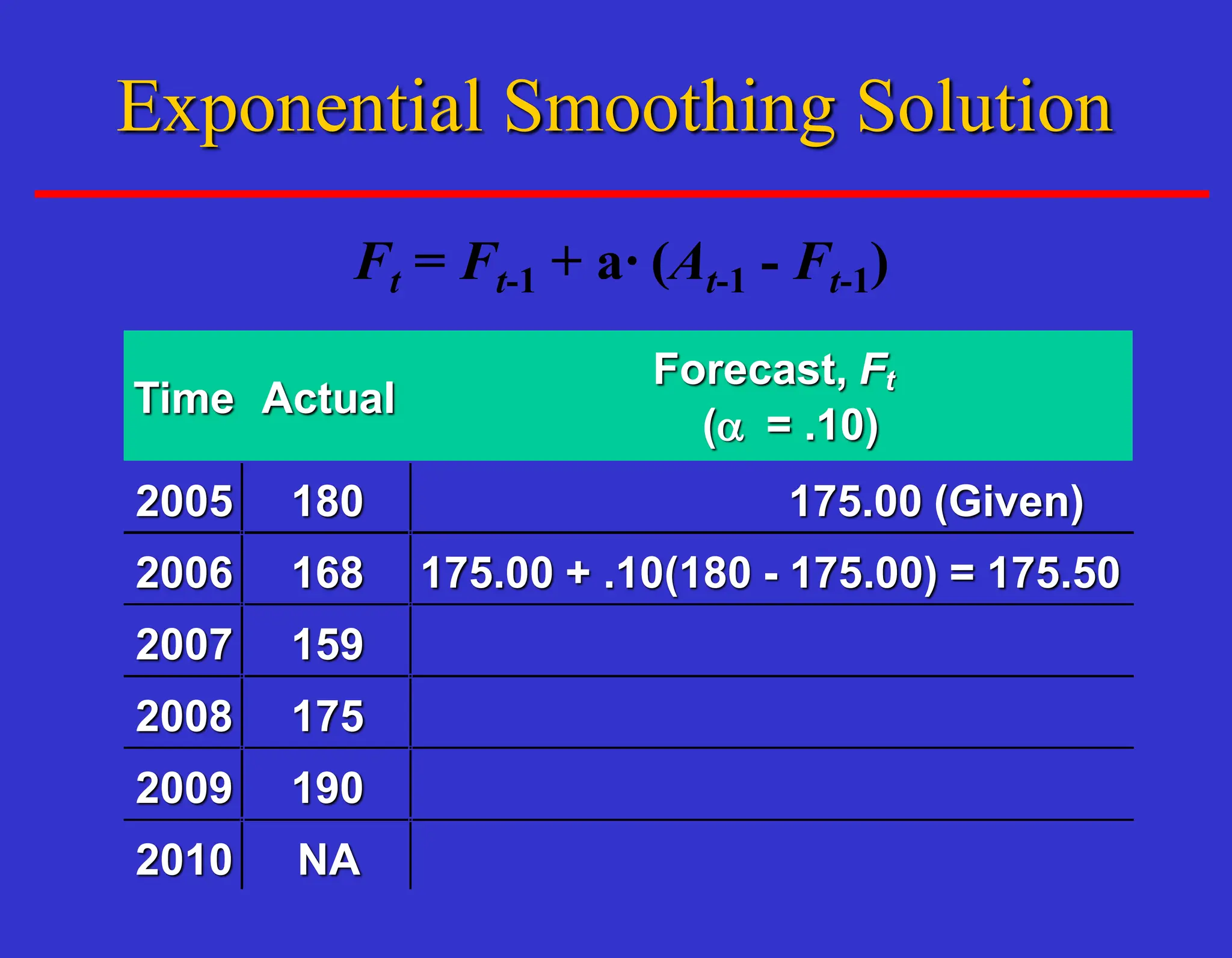
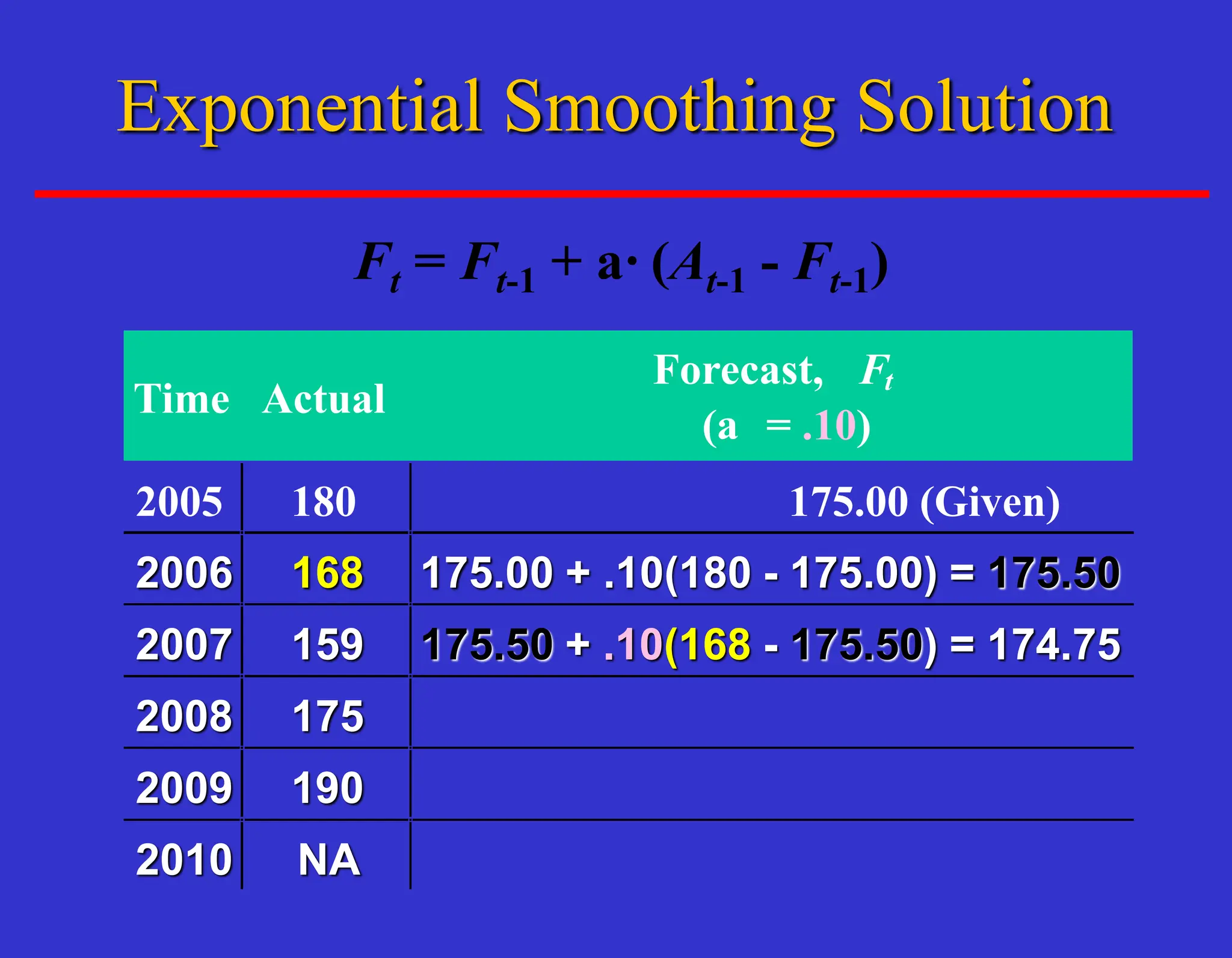
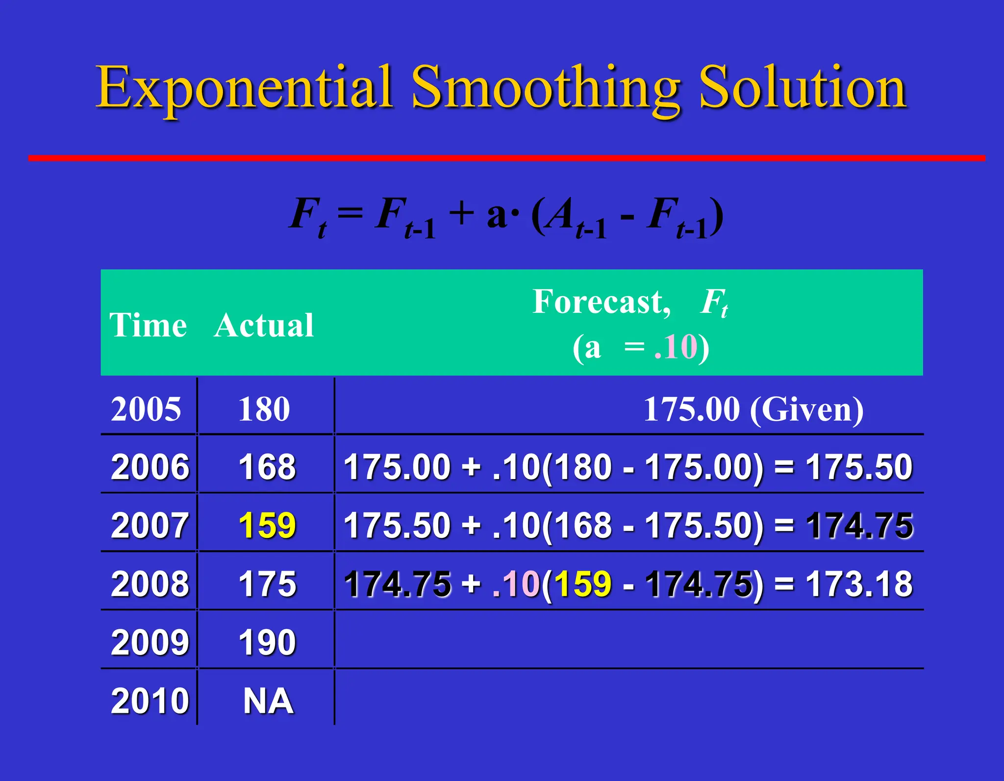
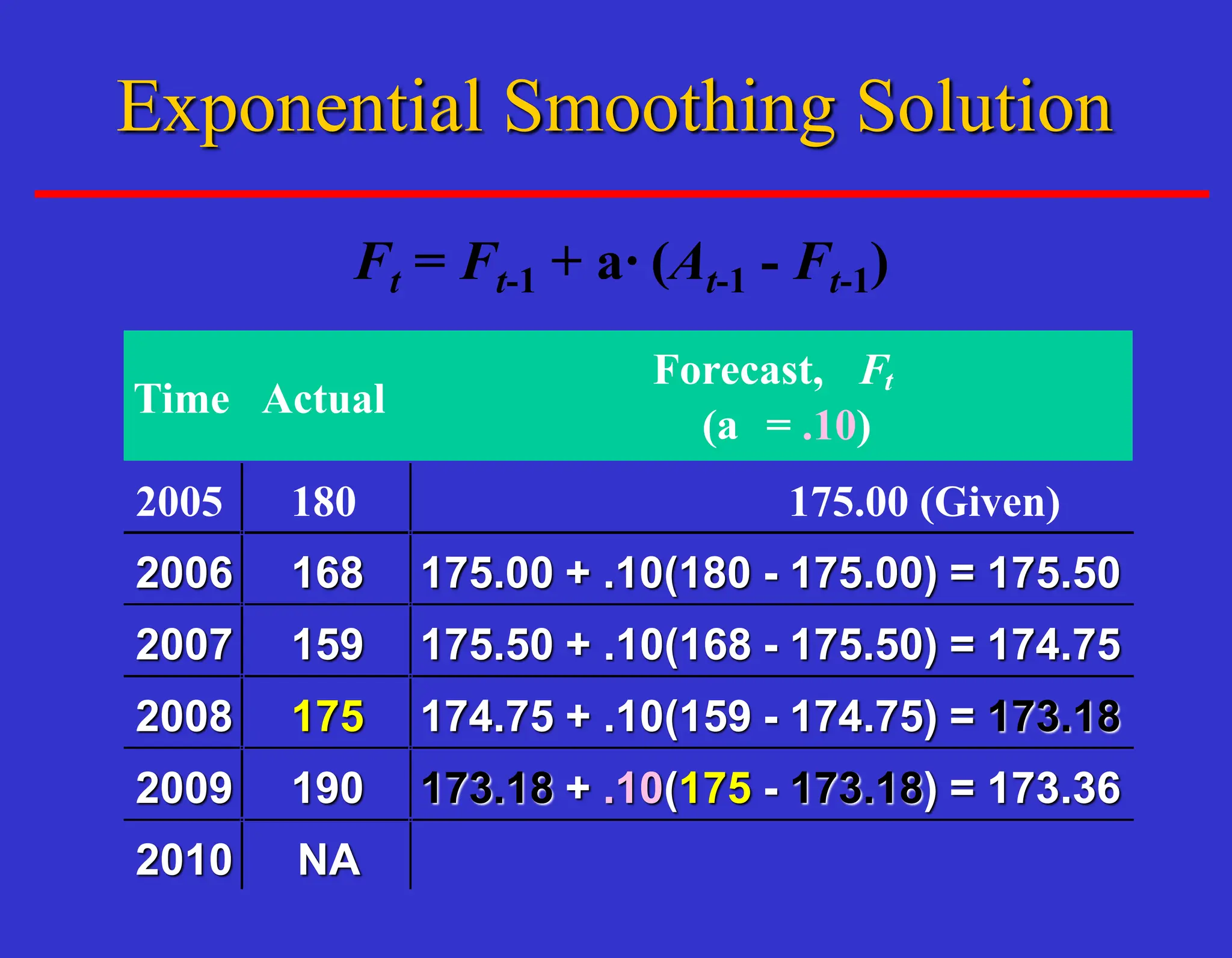
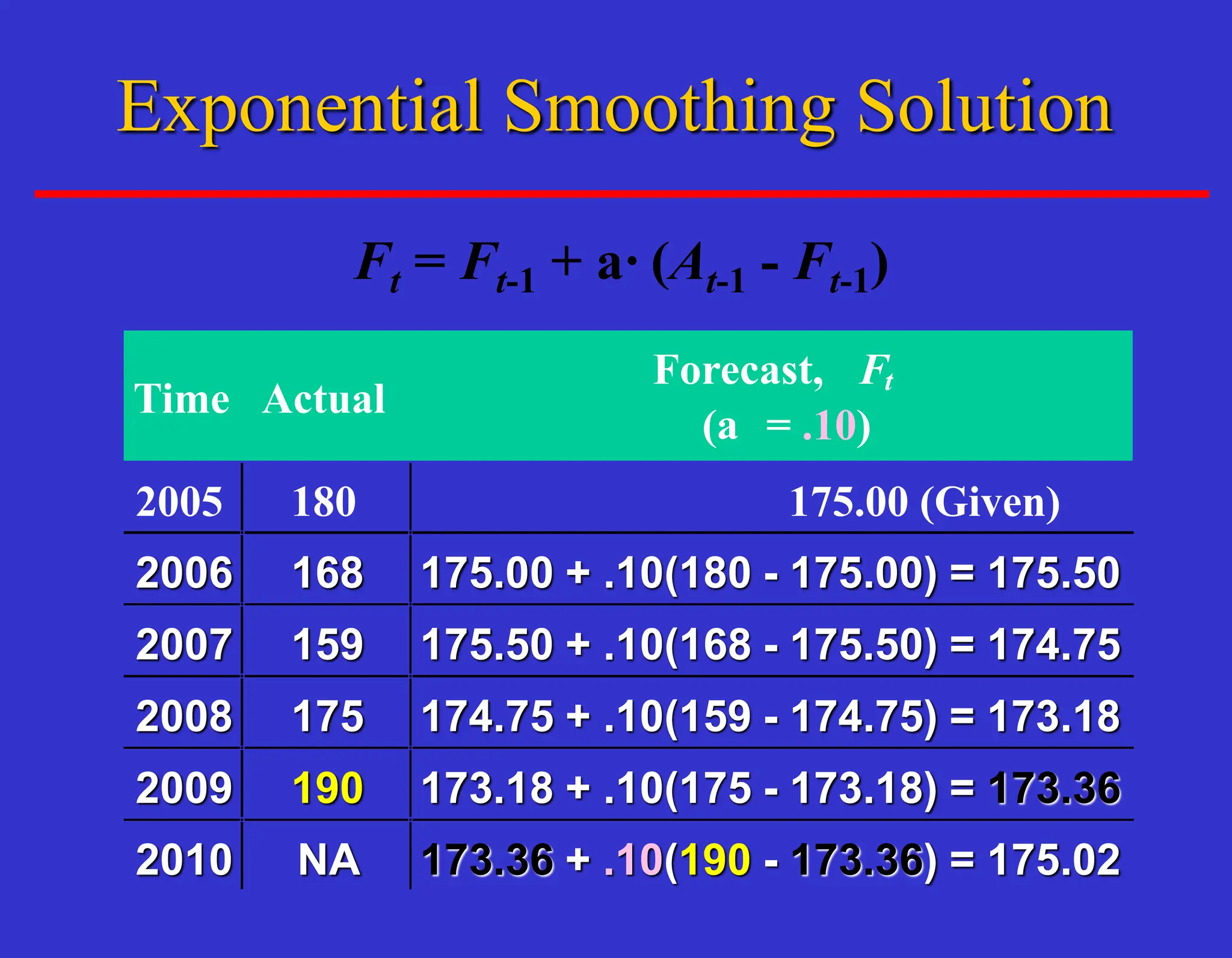
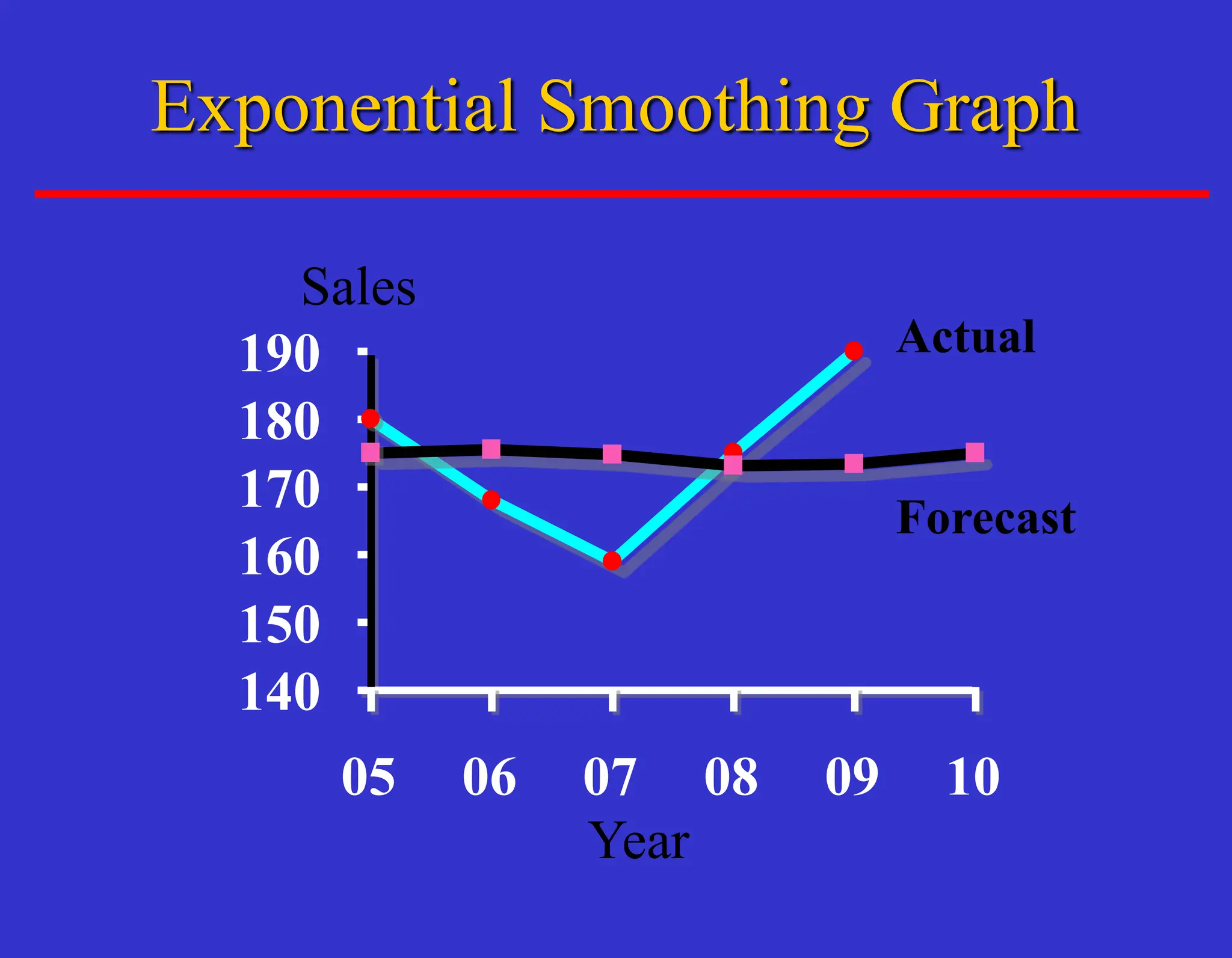
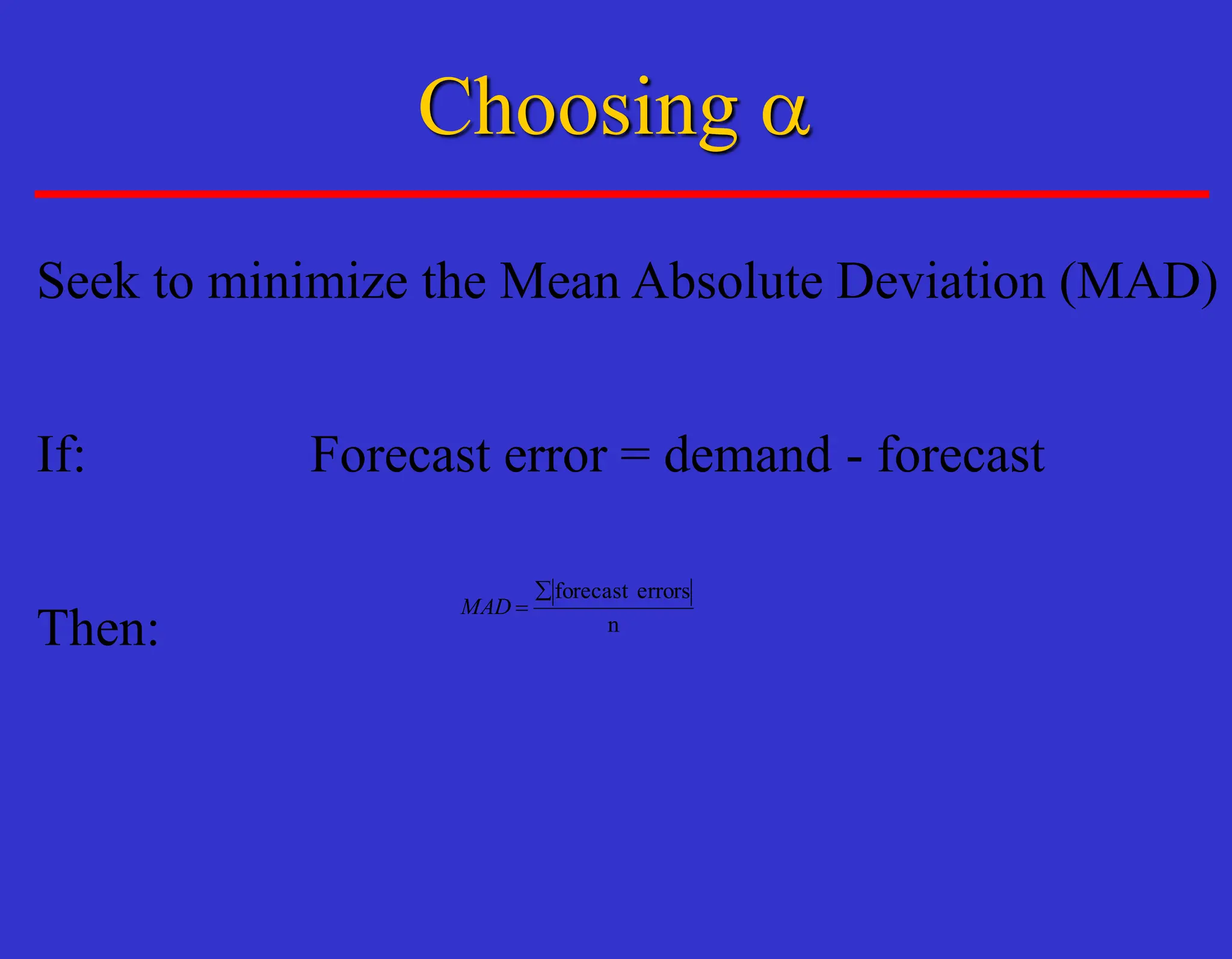
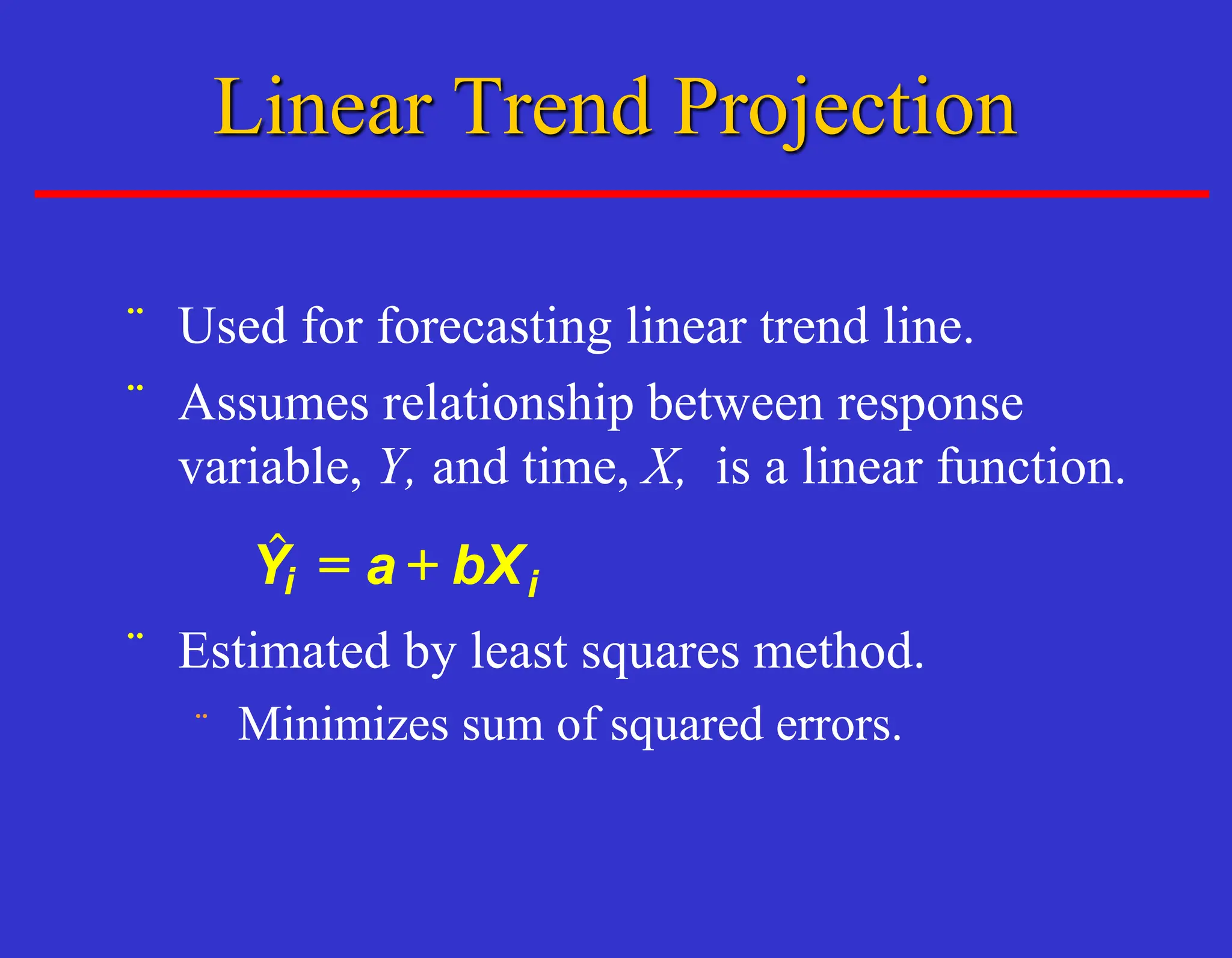
1. Operations Management
Forecasting
By
Dr. Hisham Hussein Zaher

2. Forecasting at Tupperware
¨ Each of 50 profit centers around the
world is responsible for computerized
monthly, quarterly, and 12-month sales
projections
¨ These projections are aggregated by
region, then globally at Tupperware’s
World Headquarters.

3. Tupperware - Forecast by
Consensus
¨ Although inputs come from sales,
marketing, finance, and production,
final forecasts are the consensus of all
participating managers.
¨ The final step is Tupperware’s version
of the “jury of executive opinion”.

4. What is Forecasting?
¨ Process of predicting
a future event.
¨ Underlying basis of
all business decisions.
¨ Production
¨ Inventory
¨ Personnel
¨ Facilities
Sales will
be $200
Million!

5. ¨ Short-range forecast:
¨ Up to 1 year; usually < 3 months.
¨ Job scheduling, worker assignments.
¨ Medium-range forecast:
¨ 3 months to 3 years.
¨ Sales & production planning, budgeting.
¨ Long-range forecast:
¨ 3+ years.
¨ New product planning, facility location.
Types of Forecasts by Time
Horizon

6. Short-term vs. Longer-term
Forecasting
¨ Medium/long range forecasts deal with more
comprehensive issues and support
management decisions regarding planning
and products, plants and processes.
¨ Short-term forecasting usually employs
different methodologies than longer-term
forecasting.
¨ Short-term forecasts tend to be more accurate
than longer-term forecasts.

7. Influence of Product Life Cycle
¨ Stages of introduction & growth
require longer forecasts than maturity
and decline.
¨ Forecasts useful in projecting:
¨ staffing levels,
¨ inventory levels, and
¨ factory capacity
as product passes through stages.

8. Types of Forecasts
¨ Economic forecasts:
¨ Address business cycle.
¨ e.g., inflation rate, money supply etc.
¨ Technological forecasts:
¨ Predict technological change.
¨ Predict new product sales.
¨ Demand forecasts:
¨ Predict existing product sales.

9. )
Seven Steps in Forecasting
¨ Determine the use of the forecast.
¨ Select the items to be forecast.
¨ Determine the time horizon of the
forecast.
¨ Select the forecasting model(s).
¨ Gather the data.
¨ Make the forecast.
¨ Validate and implement results.

10. Realities of Forecasting
¨ Forecasts are seldom perfect.
¨ Most forecasting methods assume that
there is some underlying stability in the
system.
¨ Both product family and aggregated
product forecasts are more accurate
than individual product forecasts.

11. Forecasting Approaches
¨ Used when situation is
‘stable’ & historical
data exist.
¨ Existing products
¨ Current technology
¨ Involves mathematical
techniques.
¨ e.g. forecasting sales
of LED color
televisions.
Quantitative Methods
¨ Used when situation is
vague & little data
exist.
¨ New products
¨ New technology
¨ Involves intuition and
experience.
¨ e.g. forecasting sales
on Internet.
Qualitative Methods

12. Overview of Qualitative Methods
¨ Jury of executive opinion
¨ Pool opinions of high-level executives,
sometimes augment by statistical models.
¨ Sales force composite
¨ estimates from individual salespersons are
reviewed for reasonableness, then aggregated.
¨ Delphi method
¨ Panel of experts, queried iteratively.
¨ Consumer Market Survey
¨ Ask the customer.

13. ¨ Involves small group of high-level managers.
“Group estimates demand by working
together”.
¨ Combines managerial experience with
statistical models.
¨ Relatively quick.
¨ ‘Group-think’
disadvantage.
Jury of Executive Opinion

14. Sales Force Composite
¨ Each salesperson
projects their sales.
¨ Combined at district &
national levels.
¨ Sales rep’s know
customers’ wants.
¨ Tends to be overly
optimistic.
Sales

15. Delphi Method
¨ Iterative group
process.
¨ 3 types of people:
¨ Decision makers.
¨ Staff.
¨ Respondents.
¨ Reduces ‘group-
think’.
Respondents
Staff
Decision Makers
(Sales?)
(What
will sales
be?
survey)
(Sales will be 45, 50, 55)
(Sales will be 50!)

16. Consumer Market Survey
¨ Ask customers
about purchasing
plans.
¨ What consumers
say, and what they
actually do are
often different.
¨ Sometimes
difficult to answer.
How many hours will
you use the Internet
next week?
© 1995 Corel
Corp.

17. Overview of Quantitative Approaches
¨ Naïve approach
¨ Moving averages
¨ Exponential
smoothing
¨ Trend projection
¨ Linear regression
Time-series
Models
Causal
models

18. Quantitative Forecasting Methods
(Non-Naive)
Quantitative
Forecasting
Linear
Regression
Causal
Models
Exponential
Smoothing
Moving
Average
Time Series
Models
Trend
Projection

19. ¨ Set of evenly spaced numerical data.
¨ Obtained by observing response variable at
regular time periods.
¨ Forecast based only on past values.
¨ Assumes that factors influencing past,
present, & future will continue.
¨ Example
Year: 2005 2006 2007 2008 2009
Sales: 78.7 63.5 89.7 93.2 92.1
What is a Time Series?

20. Trend
Seasonal
Cyclical
Random
Time Series Components

21. ¨ Persistent, overall upward or downward
pattern.
¨ Due to population, technology etc...
¨ Several years duration.
Mo., Qtr., Yr.
Response
Trend Component

22. ¨ Repeating up & down movements.
¨ Due to interactions of factors influencing
economy.
¨ Usually 2-10 years duration.
Mo., Qtr., Yr.
Response
Cycle
B
Cyclical Component

23. ¨ Regular pattern of up & down
fluctuations.
¨ Due to weather, customs etc.
¨ Occurs within 1 year.
Mo., Qtr.
Response
Summer
Seasonal Component

24. ¨ Erratic, unsystematic, ‘residual’
fluctuations.
¨ Due to random variation or unforeseen
events.
¨ Union strike
¨ Tornado
¨ Short duration &
no repeating.
Random Component

25. Naive Approach
¨ Assumes demand in next
period is the same as
demand in most recent
period.
¨ e.g., If May sales were 48,
then June sales will be 48.
¨ Sometimes cost effective
& efficient.

26. ¨ MA is a series of arithmetic means
¨ Used if little or no trend
¨ Used often for smoothing
¨ Provides overall impression of data over
time
¨ Equation:
MA
n
n
=
 Demand in Previous Periods
Moving Average Method

27. You’re manager of a museum store that sells
historical replicas. You want to forecast sales
in (000) for 2010 using a 3-period moving
average.
2005 4
2006 6
2007 5
2008 3
2009 7
Moving Average Example

28. Time
Response
Yi
Moving Total
(n = 3)
Moving
Avg. (n = 3)
2005 4
2006 6
2007 5
NA NA
NA NA
NA NA
2008 3
2009 7
2010 NA
4 + 6 + 5 = 15
Moving Average Solution

29. Time
Response
Yi
Moving Total
(n = 3)
Moving
Avg. (n = 3)
2005 4 NA NA
2006 6 NA NA
2007 5 NA NA
2008 3 4 + 6 + 5 = 15 15/3 = 5.0
2009 7
2010 NA
6 + 5 + 3 = 14
Moving Average Solution

30. Time
Response
Yi
Moving Total
(n = 3)
Moving
Avg. (n = 3)
2005 4 NA NA
2006 6 NA NA
2007 5 NA NA
2008 3 4 + 6 + 5 = 15 15/3 = 5.0
2009 7 6 + 5 + 3 = 14 14/3 = 4.7
2010 NA 5 + 3 + 7 = 15 15/3 = 5.0
Moving Average Solution

31. Year
Sales
0
2
4
6
8
05 06 07 08 09 10
Actual
Forecast
Moving Average Graph

32. ¨ Used when trend is present.
¨ Older data usually less important.
¨ Weights based on intuition.
¨ Equation:
WMA =

(Weight for period n) (Demand in period n)
Weights
Weighted Moving Average
Method

33. ¨ Increasing n makes forecast less
sensitive to changes.
¨ Do not forecast trend well.
¨ Require much historical
data.
Disadvantages of
Moving Average Method

34. ¨ Form of weighted moving average.
¨ Weights decline exponentially.
¨ Most recent data weighted most.
¨ Requires smoothing constant (a).
¨ Ranges from 0 to 1.
¨ Subjectively chosen.
¨ Involves little record keeping of past
data.
Exponential Smoothing Method

35. ¨ Ft = a·At - 1 + a·(1-a)·At - 2 + a·(1- a)2·At - 3
+ a·(1- a)3·At - 4 + ... + (1- a)t-1·A0
¨ Ft = Forecast value
¨ At = Actual value
 a = Smoothing constant
¨ Ft = Ft-1 + a·(At-1 - Ft-1)
¨ Use for computing forecast.
Exponential Smoothing
Equations

36. You’re organizing a Kwanza meeting. You
want to forecast attendance for 2010 using
exponential smoothing
(a = .10). The 2005 forecast was 175.
2005 180
2006 168
2007 159
2008 175
2009 190
Exponential Smoothing Example

37. Ft = Ft-1 + a· (At-1 - Ft-1)
Time Actual
Forecast, Ft
(a = .10)
2005 180 175.00 (Given)
2006 168
2007 159
2008 175
2009 190
2010 NA
175.00 +
Exponential Smoothing Solution

38. Ft = Ft-1 + a· (At-1 - Ft-1)
Time Actual
Forecast, Ft
(a = .10)
2005 180 175.00 (Given)
2006 168 175.00 + .10(
2007 159
2008 175
2009 190
2010 NA
Exponential Smoothing Solution

39. Ft = Ft-1 + a· (At-1 - Ft-1)
Time Actual
Forecast, Ft
(a = .10)
2005 180 175.00 (Given)
2006 168 175.00 + .10(180 -
2007 159
2008 175
2009 190
2010 NA
Exponential Smoothing Solution

40. Ft = Ft-1 + a· (At-1 - Ft-1)
Time Actual
Forecast, Ft
(a = .10)
2005 180 175.00 (Given)
2006 168 175.00 + .10(180 - 175.00)
2007 159
2008 175
2009 190
2010 NA
Exponential Smoothing Solution

41. Ft = Ft-1 + a· (At-1 - Ft-1)
Time Actual
Forecast, Ft
(a = .10)
2005 180 175.00 (Given)
2006 168 175.00 + .10(180 - 175.00) = 175.50
2007 159
2008 175
2009 190
2010 NA
Exponential Smoothing Solution

42. Ft = Ft-1 + a· (At-1 - Ft-1)
Time Actual
Forecast, Ft
(a = .10)
2005 180 175.00 (Given)
2006 168 175.00 + .10(180 - 175.00) = 175.50
2007 159 175.50 + .10(168 - 175.50) = 174.75
2008 175
2009 190
2010 NA
Exponential Smoothing Solution

43. Ft = Ft-1 + a· (At-1 - Ft-1)
Time Actual
Forecast, Ft
(a = .10)
2005 180 175.00 (Given)
2006 168 175.00 + .10(180 - 175.00) = 175.50
2007 159 175.50 + .10(168 - 175.50) = 174.75
2008 175
2009 190
2010 NA
174.75 + .10(159 - 174.75) = 173.18
Exponential Smoothing Solution

44. Ft = Ft-1 + a· (At-1 - Ft-1)
Time Actual
Forecast, Ft
(a = .10)
2005 180 175.00 (Given)
2006 168 175.00 + .10(180 - 175.00) = 175.50
2007 159 175.50 + .10(168 - 175.50) = 174.75
2008 175 174.75 + .10(159 - 174.75) = 173.18
2009 190 173.18 + .10(175 - 173.18) = 173.36
2010 NA
Exponential Smoothing Solution

45. Ft = Ft-1 + a· (At-1 - Ft-1)
Time Actual
Forecast, Ft
(a = .10)
2005 180 175.00 (Given)
2006 168 175.00 + .10(180 - 175.00) = 175.50
2007 159 175.50 + .10(168 - 175.50) = 174.75
2008 175 174.75 + .10(159 - 174.75) = 173.18
2009 190 173.18 + .10(175 - 173.18) = 173.36
2010 NA 173.36 + .10(190 - 173.36) = 175.02
Exponential Smoothing Solution

46. Year
Sales
140
150
160
170
180
190
05 06 07 08 09 10
Actual
Forecast
Exponential Smoothing Graph

47. Choosing a
Seek to minimize the Mean Absolute Deviation (MAD)
If: Forecast error = demand - forecast
Then: n
errors
forecast

=
MAD

48. ¨ Used for forecasting linear trend line.
¨ Assumes relationship between response
variable, Y, and time, X, is a linear function.
¨ Estimated by least squares method.
¨ Minimizes sum of squared errors.
$i
Y a bXi
= +
Linear Trend Projection

49. $
Y a bX
i i
= +
$
Y a bX
i i
= +
b > 0
b < 0
a
a
Y
Time, X
Linear Trend Projection Model

50. Time
Sales
0
1
2
3
4
04 05 06 07 08
Sales vs. Time
Scatter Diagram

51. Least Squares Equations
Equation: i
i bx
a
Ŷ +
=
Slope:
 


=

=




=
x
n
x
y
x
n
y
x
b
i
n
i
i
i
n
i
Y-Intercept: x
b
y
a 
=

52. Xi Yi Xi
2
Yi
2
XiYi
X1 Y1 X1
2
Y1
2
X1Y1
X2 Y2 X2
2
Y2
2
X2Y2
: : : : :
Xn Yn Xn
2
Yn
2
XnYn
SXi SYi SXi
2
SYi
2
SXiYi
Computation Table

53. You’re a marketing analyst for Hasbro Toys.
You gather the following data:
YearSales (Units)
2004 1
2005 1
2006 2
2007 2
2008 4
What is the trend equation?
Linear Trend Projection Example

54. Y X
i i
= +
a b
¨ Shows linear relationship between dependent &
explanatory variables.
¨ Example: Sales & advertising (not time)
Dependent
(response) variable
Independent
(explanatory) variable
Slope
Y-intercept
^
Linear Regression Model

55. Y
X
Y a i
+
^
i i
b X
i = + Error
Error
Observed value
Y a b X
= +
Regression line
Linear Regression Model

56. Linear Regression Equations
Equation: i
i bx
a
Ŷ +
=
Slope:
 


=

=




=
x
n
x
y
x
n
y
x
b
i
n
i
i
i
n
i
Y-Intercept: x
b
y
a 
=

57. Xi Yi Xi
2
Yi
2
XiYi
X1 Y1 X1
2
Y1
2
X1Y1
X2 Y2 X2
2
Y2
2
X2Y2
: : : : :
Xn Yn Xn
2
Yn
2
XnYn
SXi SYi SXi
2
SYi
2
SXiYi
Computation Table

58. ¨ Slope (b)
¨ Estimated Y changes by b for each 1 unit
increase in X.
¨ If b = 2, then sales (Y) is expected to increase
by 2 for each 1 unit increase in advertising (X).
¨ Y-intercept (a)
¨ Average value of Y when X = 0.
¨ If a = 4, then average sales (Y) is expected to
be 4 when advertising (X) is 0.
Interpretation of Coefficients

59. ¨ Answers: ‘how strong is the linear
relationship between the variables?.’
¨ Coefficient of correlation Sample
correlation coefficient denoted r.
¨ Values range from -1 to +1.
¨ Measures degree of association.
Correlation

60. Sample Coefficient of
Correlation



































=
 
 
  
2
2
2
2
y
y
n
x
x
n
y
x
y
x
n
r

61. -1.0 +1.0
0
Perfect
Positive
Correlation
Increasing degree of
negative correlation
-.5 +.5
Perfect
Negative
Correlation
No
Correlation
Increasing degree of
positive correlation
Coefficient of Correlation Values

62. r = 1 r = -1
r = .89 r = 0
Y
X
Yi = a + b Xi
^
Y
X
Y
X
Y
X
Yi = a + b Xi
^ Yi = a + b Xi
^
Yi = a + b Xi
^
Coefficient of Correlation and
Regression Model

63. ¨ You want to achieve:
¨ No pattern or direction in forecast error
¨ Error = (Yi - Yi) = (Actual - Forecast)
¨ Seen in plots of errors over time
¨ Smallest forecast error
¨ Mean square error (MSE)
¨ Mean absolute deviation (MAD)
^
Guidelines for Selecting
Forecasting Model

64. Time (Years)
Error
0
Desired Pattern
Time (Years)
Error
0
Trend Not Fully
Accounted for
Pattern of Forecast Error

65. ¨ Mean Square Error (MSE)
¨ Mean Absolute Deviation (MAD)
Forecast Error Equations
n
errors
forecast
n
)
ŷ
y
(
MSE
n
i
i
i 

=

= 
=

n
|
errors
forecast
|
n
|
ŷ
y
|
MAD
n
i
i
i 

=

= 
=

66. You’re a marketing analyst for Hasbro Toys. You’ve forecast sales with
a linear model & exponential smoothing. Which model do you use?
Actual Linear Model Exponential
Smoothing
Year Sales Forecast Forecast (.9)
2004 1 0.6 1.0
2005 1 1.3 1.0
2006 2 2.0 1.9
2007 2 2.7 2.0
2008 4 3.4 3.8
Selecting Forecasting Model
Example

67. Year
^
Yi Yi
^
2004 1 0.6 0.4 0.16 0.4
2005 1 1.3 -0.3 0.09 0.3
2006 2 2.0 0.0 0.00 0.0
2007 2 2.7 -0.7 0.49 0.7
2008 4 3.4 0.6 0.36 0.6
Total 0.0 1.10 2.0
Error Error2 |Error|
Linear Model Evaluatin

68. Year
^
Yi Yi
^
2004 1 0.6 0.4 0.16 0.4
2005 1 1.3 -0.3 0.09 0.3
2006 2 2.0 0.0 0.00 0.0
2007 2 2.7 -0.7 0.49 0.7
2008 4 3.4 0.6 0.36 0.6
Total 0.0 1.10 2.0
MSE = Error2 / n = 1.10 / 5 = .220
MAD =  |Error| / n = 2.0 / 5 = .400
Error Error2 |Error|
Linear Model Evaluation

69. Year Yi Yi
2004 1 1.0 0.0 0.00 0.0
2005 1 1.0 0.0 0.00 0.0
2006 2 1.9 0.1 0.01 0.1
2007 2 2.0 0.0 0.00 0.0
2008 4 3.8 0.2 0.04 0.2
Total 0.3 0.05 0.3
^
MSE = Error2 / n = 0.05 / 5 = 0.01
MAD = |Error| / n = 0.3 / 5 = 0.06
Error Error2 |Error|
Exponential Smoothing Model
Evaluation