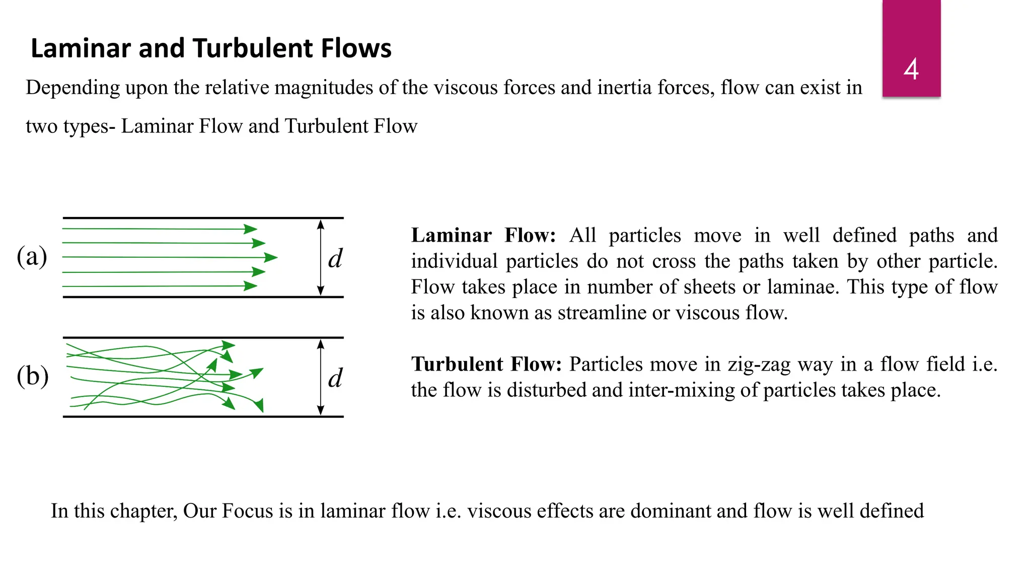
1) The document discusses viscous fluid flow through circular pipes and between parallel plates. It defines laminar and turbulent flow, and explores Reynold's experiment which shows the transition between these flow types.
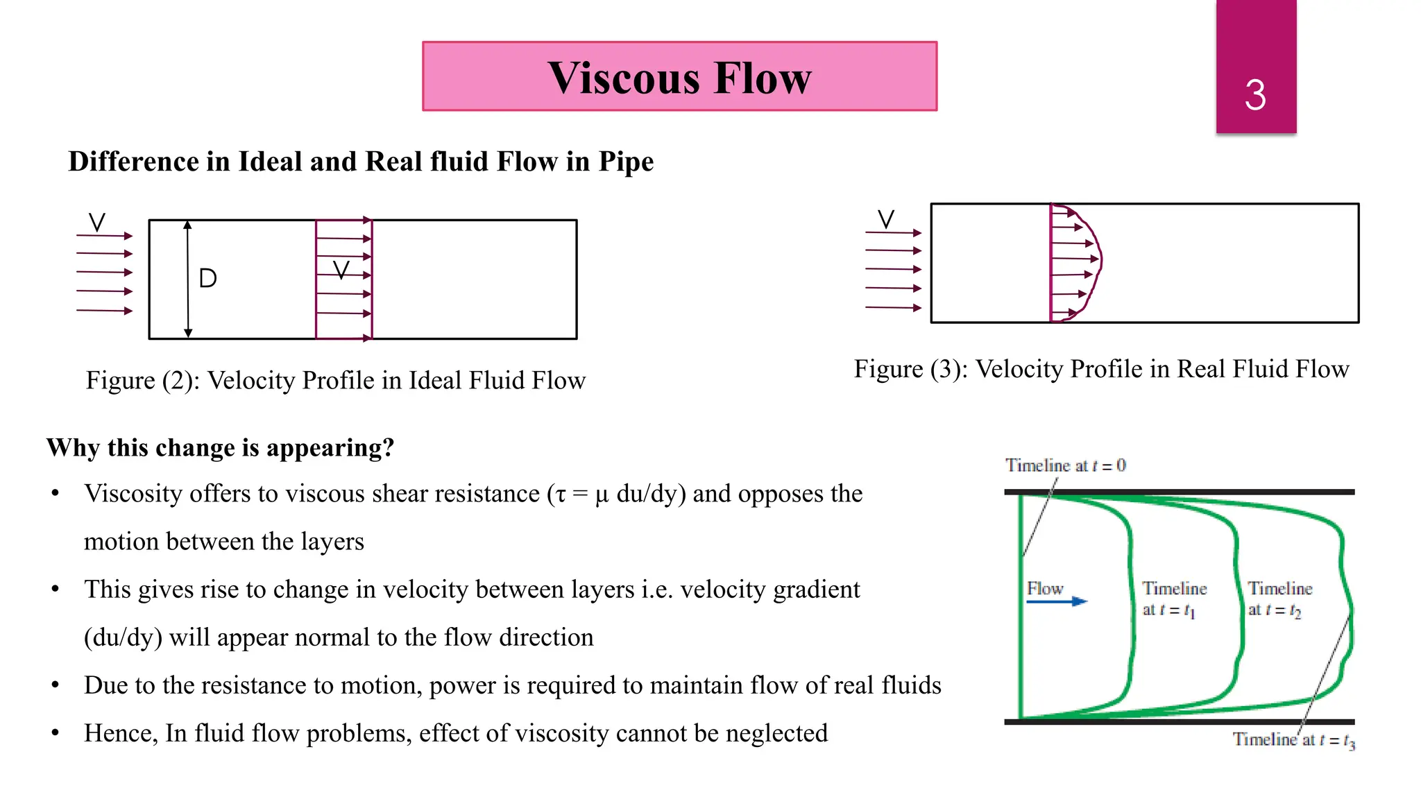
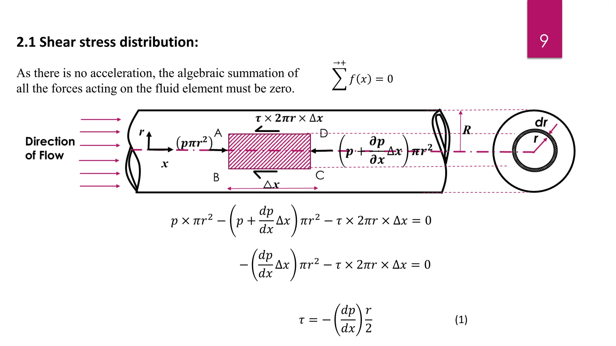
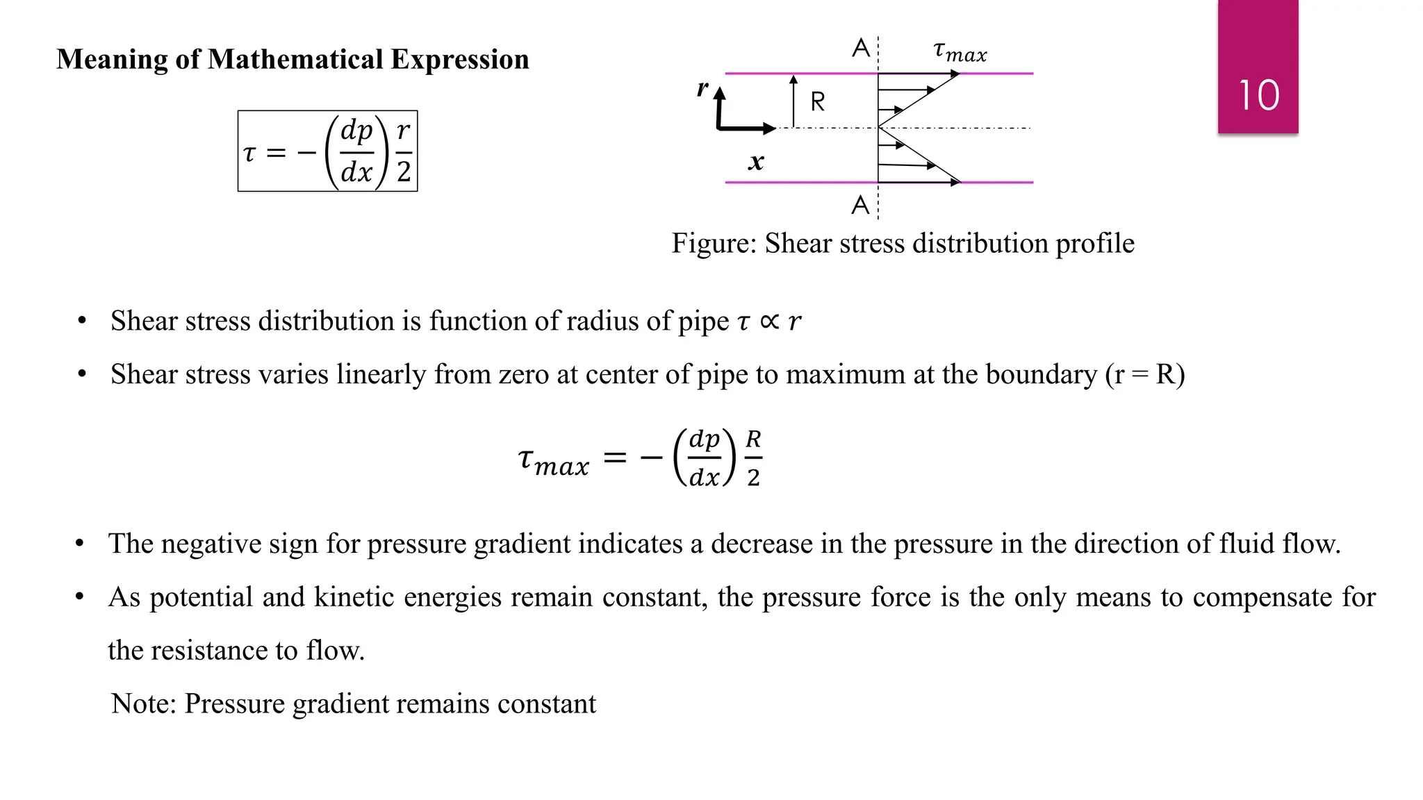
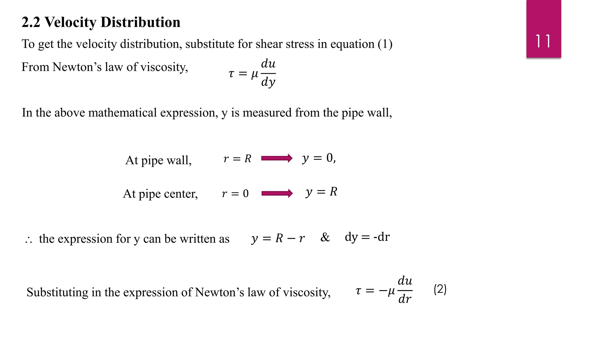
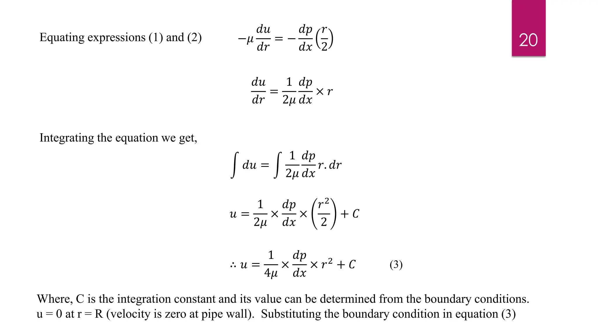
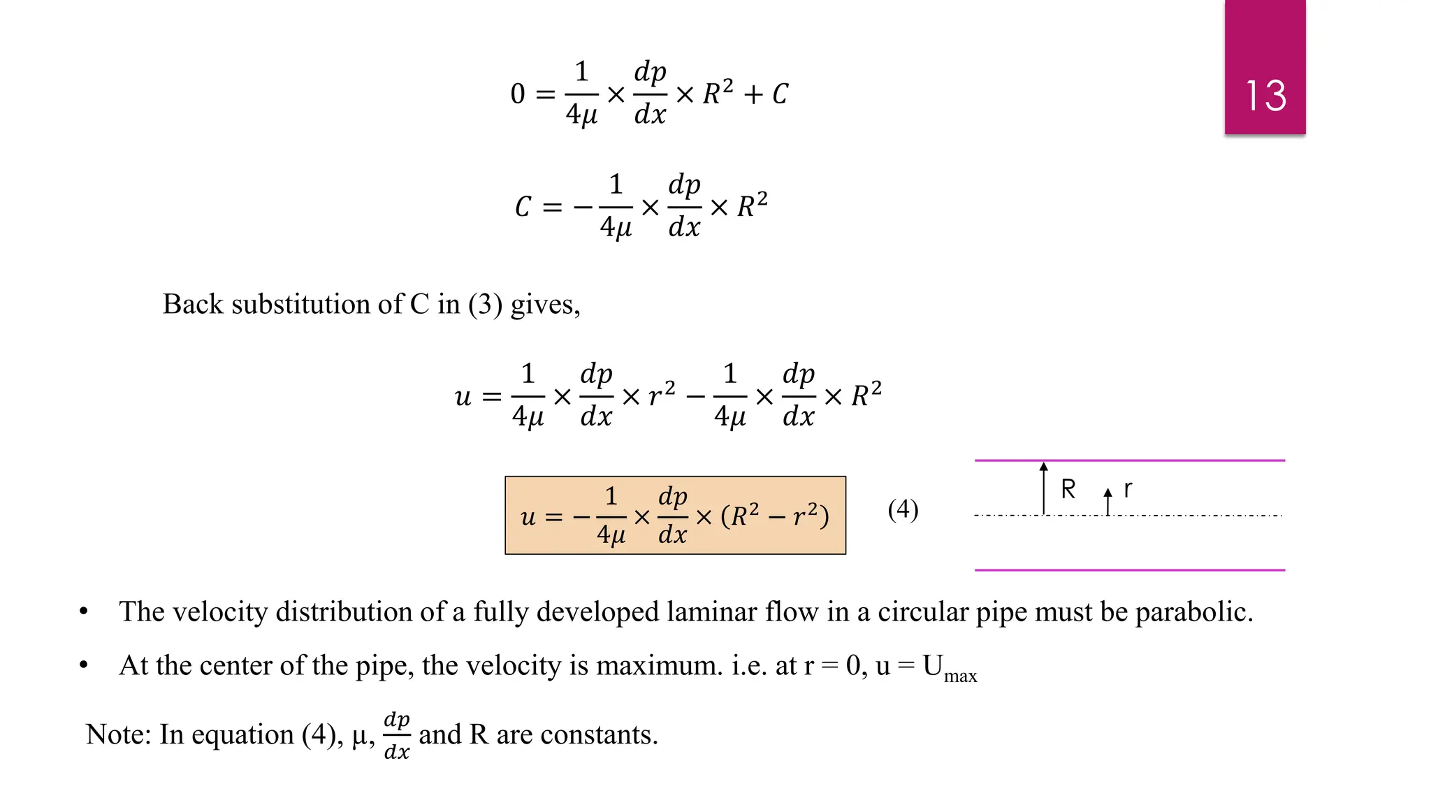
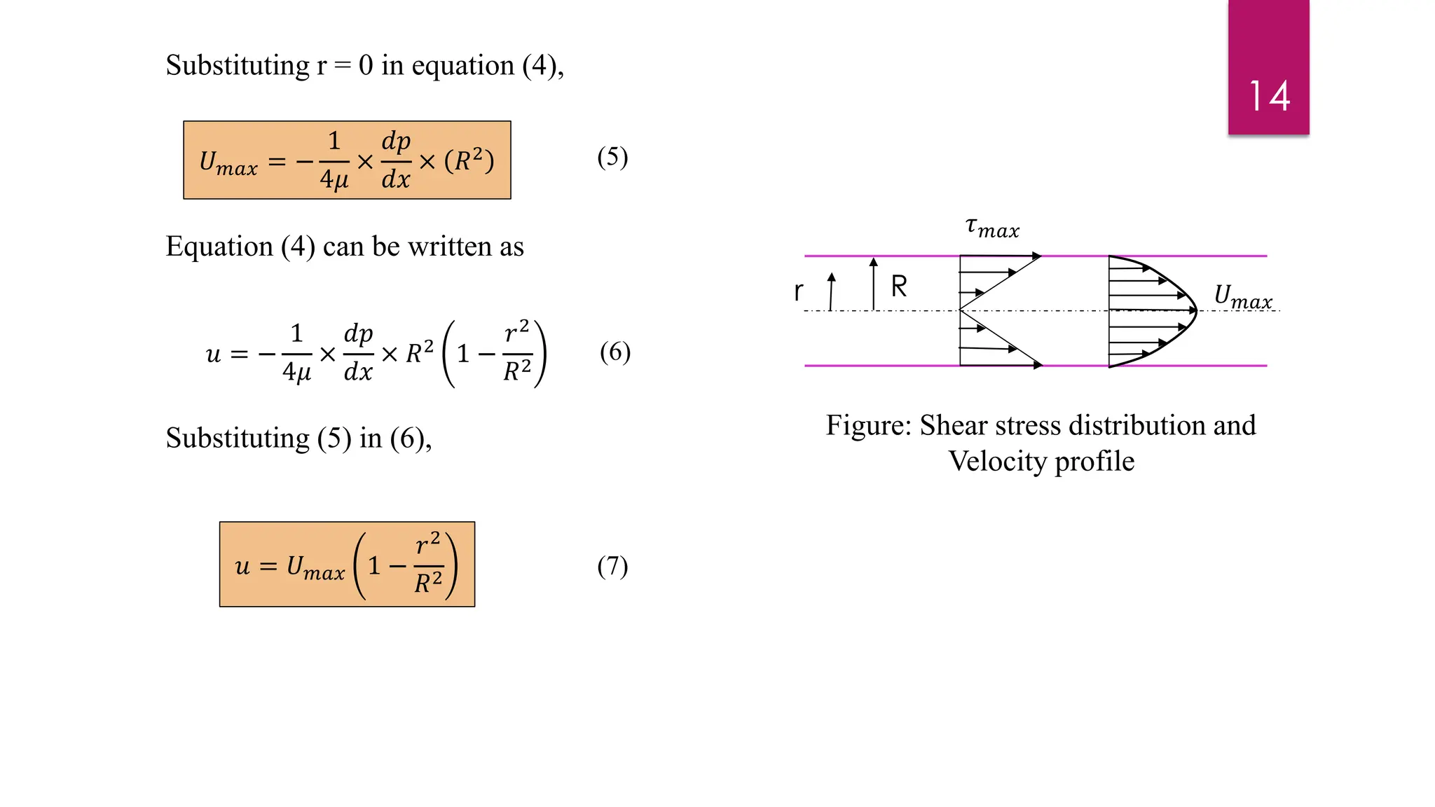
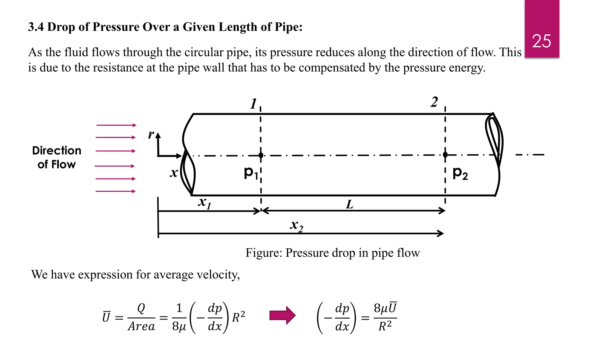
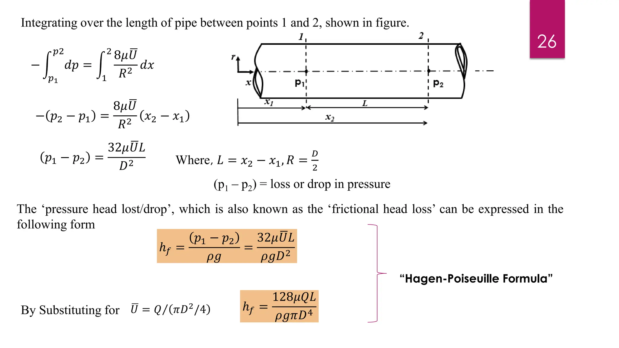
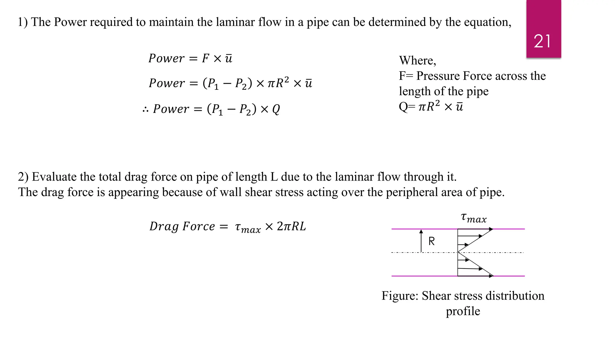
2) Mathematical expressions are derived for shear stress distribution, velocity distribution, the ratio of maximum to average velocity, and pressure drop over a given pipe length. Shear stress and velocity are shown to vary parabolically from the pipe wall to center.
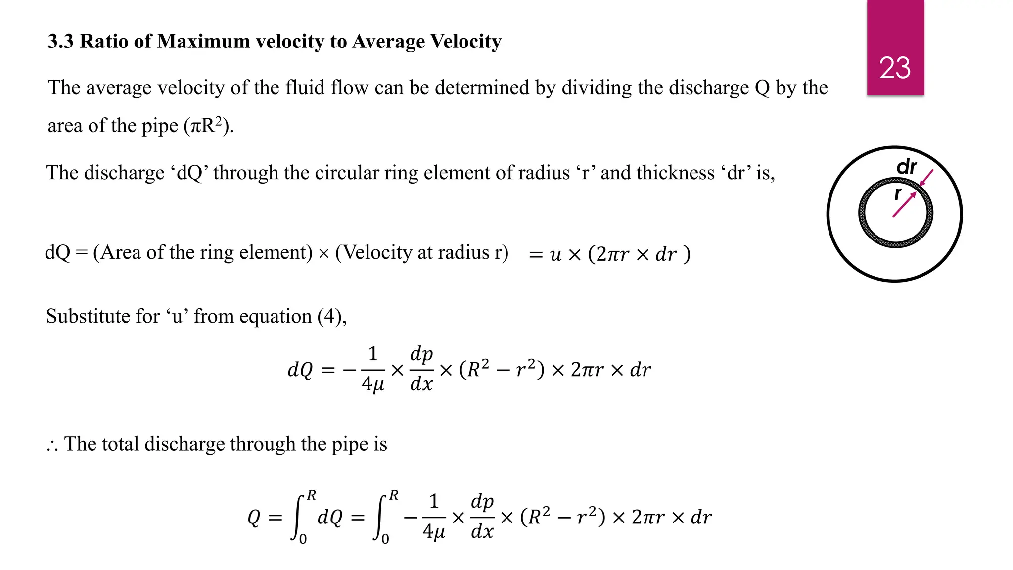
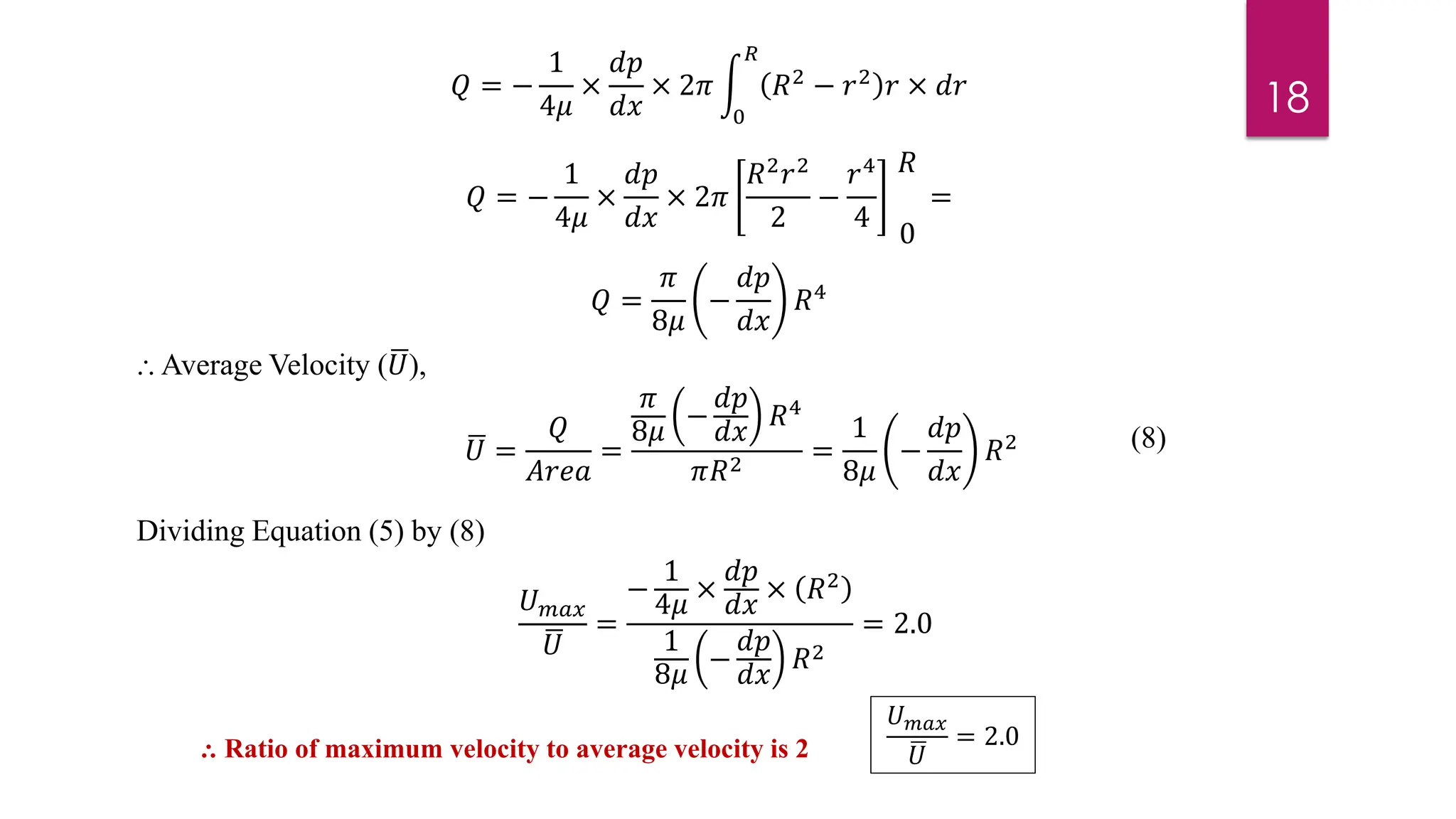
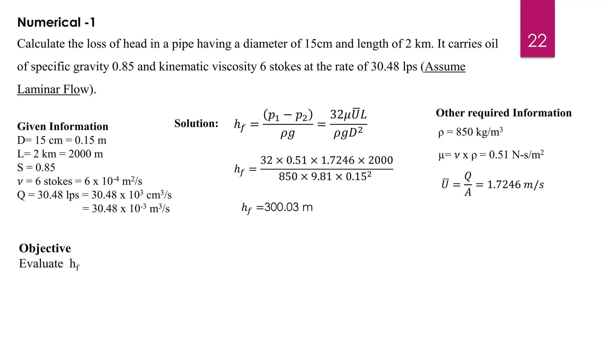
3) Key results shown are that velocity distribution is parabolic, the ratio of maximum to average velocity is 2, and the pressure drop can be calculated using the Hagen-Poiseuille formula.
![5
1) Reynolds’s Experiment:
O. Reynold, a British professor demonstrated that a laminar flow changes to turbulent flow
Figure: Reynolds Dye Experimental setup and Observed dye streak lines [1]
Q V](https://image.slidesharecdn.com/009apptviscousflow-1new-240314062358-9e09f64f/75/009a-PPT-Viscous-Flow-1-New-pdf-5-2048.jpg)
![Observations from the Reynold’s Dye Experiment
6
For general case, transition of flow is function of
• Velocity of fluid (V)
• Diameter of the pipe (V)
• Viscosity of the fluid (𝜇)
• Density of Fluid (ρ)
Figure: Time dependence of fluid velocity at a point [1]
𝑉𝐴 = 𝑢 Ƹ
𝑖
𝑉𝐴 = 𝑢 Ƹ
𝑖 + 𝑣 Ƹ
𝑗 + 𝑤
𝑘](https://image.slidesharecdn.com/009apptviscousflow-1new-240314062358-9e09f64f/75/009a-PPT-Viscous-Flow-1-New-pdf-6-2048.jpg)
![ρ = Density of Fluid,
Vavg= Average Velocity,
D= Diameter of Pipe,
µ= Dynamic Viscosity
𝑅𝑒 =
𝜌𝑉
𝑎𝑣𝑔𝐷
𝜇
For a flow in circular pipe,
If Re < 2000, the flow is said to be laminar
If Re > 4000, the flow is said to be turbulent
If 2000 < Re < 4000, in transition from laminar to turbulent
Identifying the type of flow from Reynolds Number
Critical Reynolds Number: It is magnitude of Reynolds Number below
which the flow is definitely laminar.
7
Figure: Laminar and Turbulent
flow regimes in candle smoke [3]](https://image.slidesharecdn.com/009apptviscousflow-1new-240314062358-9e09f64f/75/009a-PPT-Viscous-Flow-1-New-pdf-7-2048.jpg)
![15
Figure: Changes in velocity profile and pressure changes along the flow in pipe [2]](https://image.slidesharecdn.com/009apptviscousflow-1new-240314062358-9e09f64f/75/009a-PPT-Viscous-Flow-1-New-pdf-15-2048.jpg)
![28
End of Session-1
Figure: Shear stress distribution and typical velocity profiles for fluid flow in a pipe [1].](https://image.slidesharecdn.com/009apptviscousflow-1new-240314062358-9e09f64f/75/009a-PPT-Viscous-Flow-1-New-pdf-28-2048.jpg)