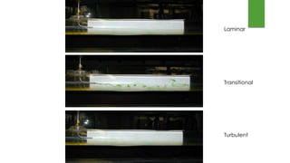
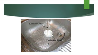
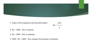
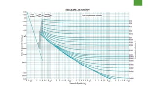
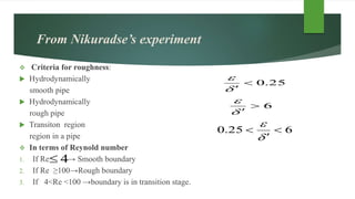
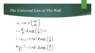
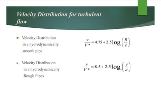
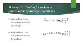
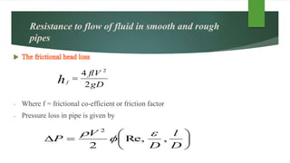
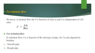
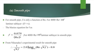
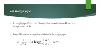
This document provides an overview of turbulent fluid flow, including: 1) It defines laminar and turbulent flow and explains that turbulent flow occurs above a Reynolds number of 2000. 2) It describes methods for characterizing turbulence, including magnitude, intensity, and mixing length theory. 3) It discusses the universal law of the wall and how velocity is distributed in smooth and rough pipes. Friction factors depend on Reynolds number and relative roughness. 4) Experimental results from Nikuradse are presented showing relationships between friction factor and Reynolds number/relative roughness that can be used to model pressure losses in pipes.

1. Gandhinagar Institute of Technology
Subject :- Fluid Mechanics
– Pavan Narkhede [130120119111]
Darshit Panchal [130120119114]
Topic :- Turbulent Flow
:
Prof.Jyotin kateshiya
MECHANICAL ENGINEERING
4th - B : 2

2. INTRODUCTION:
 Laminar Flow: In this type of flow, fluid particles moves along smooth straight parallel
paths in layers or laminas, with one layer gliding smoothly over an adjacent layer, the paths
of individual fluid particles do not cross those of neighbouring particles.
 Turbulent Flow: In turbulent flow, there is an irregular random movement of fluid in
transverse direction to the main flow. This irregular, fluctuating motion can be regarded as
superimposed on the mean motion of the fluid.

3. Laminar
Transitional
Turbulent

5.  Types of flow depend on the Reynold number , ρVd
Re = --------
µ
 Re < 2000 – flow is laminar
 Re > 2000 – flow is turbulent
 2000 < Re < 4000 – flow changes from laminar to turbulent.

6.  Magnitude of Turbulence :
- It is the degree of turbulence, and measures how strong, violent or intence
the turbulence.
- Magnitude of Turbulence = Arithmetic mean of root mean square of turbulent
fluctuations
=
=
 
2
  




t
t dt
0
2
1


7.  Intensity of turbulence :
- It is the ratio of the magnitude of turbulence to the average flow velocity at a
point in the flow field
- So, Intensity of Turbulence =
gD
lVC
h
f
f
2
2


8. From the experimental measurement on turbulent flow through pipes, it has observed
That the viscous friction associated with fluid are proportional to
(1) Length of pipe (l)
(2) Wetted perimeter (P)
(3) Vn , where V is average velocity and n is index depending on the material
(normally, commertial pipe turbulent flow n=2

9. f – friction factor
L – length of pipe
D – diameter of pipe
v – velocity of flow
OR
g
pp
hf

21


gD
lVC
h
f
f
2
2


10. Moody Diagram :
Developed to provide the friction factor for turbulent flow for various values of Relative roughness and
Reynold’s number!
From experimentation, in turbulent flow, the friction factor (or head loss) depends upon velocity of fluid
V, dia. of pipe D, density of fluid ρ, viscosity of fluid µ, wall roughness height ε.
So, f = f1 (V,D, ρ, µ, ε)
By the dimensional analysis,
, Where called relative roughness. 


0
,1 D
VD
ff 
D


12. Key points about the Moody Diagram –
1. In the laminar zone – f decreases as Nr increases!
2. 2. f = 64/Nr.
3. 3. transition zone – uncertainty – not possible to predict -
4. Beyond 4000, for a given Nr, as the relative roughness term D/ε increases (less rough), friction
factor decreases

13. 5. For given relative roughness, friction factor decreases with increasing Reynolds number till the
zone of complete turbulence
6. Within the zone of complete turbulence – Reynolds number has no affect.
7. As relative roughness increases (less rough) – the boundary of the zone of complete turbulence
shifts (increases)

14. Co-efficient of friction in terms of shear
stress :
We know, the propelling force = (p1 - p2) Ac ---- (1)
Frictional resistance in terms of shear stress = As Where = shear stress ----(2)
By comparing both equation,
(P1 – P2) = OR
( co-efficient of frictionin terms of shear stress)
0 0
V
f 2
0
2

 vu
dA
uvdA
dA
dF
t


 



15. Shear stress in turbulent flow
In turbulent flow, fluid particles moves randomly, therefore it is impossible to trace the
Paths of the moving particles and represents it mathematically

16. ub
ub
u
= mean velocity of particles moving along layer A
= mean velocity of particles moving along layer B
= -
Shear stress in turbulent flow
It is the shear stress exerted by layer A on b and known as
Reynold’s stress.
uaub
22
yk
dy
du
dy
du
dy
du
dy
du
dy
du
dy
du
tv













































t

17. Prandtl’s mixing length theory :
Prandtl’s assumed that distance between two layers in the transverse direction
(called mixing length l) such that the lumps of fluid particles from one layer could reach the other
Layer and the particles are mixed with the other layer in such a way that the momentum of the
Particles in the direction of x is same, as shown in below figure :

19. Total shear
where , (Viscosity)
n = 0 for laminar flow.
For highly turbulent flow, .
 tv 













dy
du
yk
dy
du 22














dy
du
dy
du













dy
du
dy
du

22
yk 

20. Hydrodynamically Smooth and
Rough Pipe Boundaries
 Hydronamically smooth pipe :
 The hight of roughness of pipe is less than thickness of
laminar sublayer of flowing fluid.
 K < δ′
 Hydronamically rough pipe :
 The hight of roughness of pipe is greater than the thickness
of laminar sublayer of flowing fluid.
 K > δ′

21. From Nikuradse’s experiment
 Criteria for roughness:
 Hydrodynamically
smooth pipe
 Hydrodynamically
rough pipe
 Transiton region
region in a pipe
 In terms of Reynold number
1. If Re → Smooth boundary
2. If Re ≥100→Rough boundary
3. If 4<Re <100 →boundary is in transition stage.
625.0 




25.0


6


4

22. The Universal Law of The Wall







dy
dv
yk
2
22
0

C
R
y
K
v LogV
e






 *







R
y
v LogVv e*m ax
5.2








y
Rv
LogV
V
v
e*
*
max
5.2

23. Velocity Distribution for turbulent
flow
 Velocity Distribution
in a hydrodynamically
smooth pipe
 Velocity Distribution
in a hydrodynamically
Rough Pipes








y
V
v
e
log5.25.8
*








R
V
v
e
log5.275.4
*

24. Velocity Distribution for turbulent
flow in terms of average Velocity (V)
 Velocity Distribution
in a hydrodynamically
smooth pipe
 Velocity Distribution
in a hydrodynamically
Rough Pipes








RV
V
V
e
*
5.275.1
*
log








R
V
V
e
log5.275.4
*

25. Resistance to flow of fluid in smooth and rough
pipes
- Where f = frictional co-efficient or friction factor
- Pressure loss in pipe is given by
gD
flV
hf
2
4 2








D
l
D
V
P ,Re,
2
2




26. - But friction factor
- From equation ,the friction factor f is a function of Re and ratio of ε/D.







D
f
 Re,







DD
lV
P



Re,
2
2


f
lV
DP
2
2








D
f

 Re,

27.  For laminar flow
- We know, in laminar flow the f is function of only re and it is independent of ε/D
ratio.
 For terbulent flow
- In terbulent flow, f is a function of Re and type of pipe. So f is also depend on
boudary.
a) Smooth pipe
b) Rough pipe
Re
16
f

28. (a) Smooth pipe
 For smooth pipe ,f is only a function of Re. For 4000<Re<
laminar sublayer (δ′>>ε).
- The blasius equation for f as
 ,For 4000<Re< laminar sublayer in smooth pipe.
 From Nikuradse’s experimental result for smooth pipe
5
10
 4
1
Re
079.0
f 5
10
8.0)4(Re0.2
4
1
log10
 f
f

29. (b) Rough pipe
- In rough pipe δ′<<ε, the f is only function of ratio ε/D and it is
independent of Re.
- From Nikuradse’s experimental result for rough pipe
74.12
4
1
log10








R
f

30. THANK YOU….