Dimensional Analysis - Model Theory- fluid mechanics

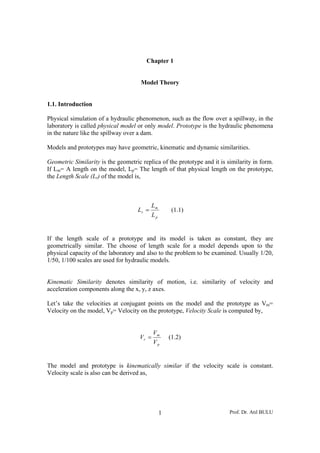
1. Prof. Dr. Atıl BULU1
Chapter 1
Model Theory
1.1. Introduction
Physical simulation of a hydraulic phenomenon, such as the flow over a spillway, in the
laboratory is called physical model or only model. Prototype is the hydraulic phenomena
in the nature like the spillway over a dam.
Models and prototypes may have geometric, kinematic and dynamic similarities.
Geometric Similarity is the geometric replica of the prototype and it is similarity in form.
If Lm= A length on the model, Lp= The length of that physical length on the prototype,
the Length Scale (Lr) of the model is,
p
m
r
L
L
L = (1.1)
If the length scale of a prototype and its model is taken as constant, they are
geometrically similar. The choose of length scale for a model depends upon to the
physical capacity of the laboratory and also to the problem to be examined. Usually 1/20,
1/50, 1/100 scales are used for hydraulic models.
Kinematic Similarity denotes similarity of motion, i.e. similarity of velocity and
acceleration components along the x, y, z axes.
Let’s take the velocities at conjugant points on the model and the prototype as Vm=
Velocity on the model, Vp= Velocity on the prototype, Velocity Scale is computed by,
p
m
r
V
V
V = (1.2)
The model and prototype is kinematically similar if the velocity scale is constant.
Velocity scale is also can be derived as,

2. Prof. Dr. Atıl BULU2
m
m
m
T
L
V = ,
p
p
p
T
L
V =
r
r
r
m
p
p
m
p
p
m
m
p
m
r
T
L
V
T
T
L
L
L
T
T
L
V
V
V
=
×=×==
(1.3)
Where Tr is the Time Scale.
p
m
r
T
T
T = (1.4)
Acceleration Scale can be derived similarly as,
2
r
r
r
r
r
p
m
r
prp
r
r
pr
pr
m
m
m
T
L
T
V
a
a
a
a
aaa
T
V
TT
VV
T
V
a
==
=
×=×=
×
×
==
(1.5)
Acceleration scale will be constant and the paths of fluid particles will be similar when
the kinematic similarity is supplied in the model and the prototype.
Dynamic similarity denotes the similarity of forces. If there is a constant ratio between
the forces on the conjugant points on the model and the prototype then the two systems is
dynamically similar.
Force Scale cons
F
F
F
p
m
r === (1.6)

3. Prof. Dr. Atıl BULU3
Generally, inertia, pressure, shearing, gravitational forces are seen on the hydraulic
models.
1.2. Similarity Conditions
Model experiments are applied for almost every important hydraulic structure. Optimum
solutions may be obtained by the observations and the measurements of the physical
event on the model which can not always be seen and understood during the analytical
solution of the structure. Hydropower plants, river improvement, coastal engineering and
also in aviation and in ship construction sectors are where the model experiments are
applied.
Similarity conditions should be supplied to find the measured values between the
conjugant points on the model and on the prototype. For instance the measured wave
height at a harbor model will correspond which height on the prototype is the question to
be answered. Dynamic Method is applied to supply the similarity conditions.
1.2.1. Dynamic Method
Dynamic Method depends on the constant variation of forces on the model and on the
prototype which is Force Scale is kept constant. Dominant forces on hydraulic structures
are Inertia, Gravitational and Viscosity forces. Denoting as Inertia Force=Fine,
Gravitational Force=Fgr, Viscosity Force=Fvis, the similarity of the ratio of forces can be
written as,
( )
( )
( )
( )
( )
( )mvis
mvis
pgr
mgr
pine
mine
F
F
F
F
F
F
== (1.7)
This equality of force ratios equation can also be written as,
( )
( )
( )
( )
( )
( )
( )
( )pine
pvis
mine
mvis
pine
pgr
mine
mgr
F
F
F
F
F
F
F
F
=
=
(1.8)
Inertia force can be defined by using Newton’s 2nd
law as,
Inertia Force = Mass × Acceleration

4. Prof. Dr. Atıl BULU4
By using the dimensions of these physical values, the dimension of the inertia force can
be derived as,
[ ] [ ] [ ] [ ]
[ ] [ ] [ ] [ ]
[ ] [ ]FF
LLTTFLF
LgF
ine
ine
ine
=
××=
××=
−− 3224
3
ρ
(1.9)
Gravitational force is the weight of the body and can be defined as,
Gravitational force = Specific weight × Volume
[ ] [ ] [ ]
[ ] [ ]FF
LFLF
gr
gr
=
×= − 33
(1.10)
The ratio of forces can be written again by using the above derived equations as,
( )
( )
( )
( )
p
p
m
m
pppp
pp
mmmm
mm
pine
pgr
mine
mgr
L
gT
L
gT
TLL
gL
TLL
gL
F
F
F
F
22
23
3
23
3
=
=
=
−−
ρ
ρ
ρ
ρ
(1.11)
Since dimension of velocity is,
[ ] [ ]
[ ]
[ ] [ ]
[ ]V
L
T
T
L
V =→=
pp
p
mm
m
LV
gL
LV
gL
2
2
2
2
=
Taking the inverse of this equation gives,

5. Prof. Dr. Atıl BULU5
p
p
m
m
gL
V
gL
V
22
= (1.12)
Since Froude number (Fr) is,
gL
V
Fr =
Equation (1.12) shows that Froude numbers calculated for the model and the prototype at
a point should be the same.
pm FrFr = (1.13)
The equality of the ratio of the gravity forces to the inertia forces results in to the equality
of Froude numbers.
Viscosity force can be defined as,
Viscosity force = Shearing stress × Area
[ ] [ ]
[ ]
[ ]2
1
L
L
LT
F
A
dy
du
F
AF
vis
vis
vis
××=
××=
×=
−
μ
μ
τ
(1.14)
The equality of the ratio of viscosity forces to inertia forces is then,
( )
( )
( )
( )
( )
( )
( )
( )
22
23
21
23
21
pp
pp
mm
mm
pppp
ppppp
mmmm
mmmmm
pine
pvis
mine
mvis
L
T
L
T
TLL
LLTL
TLL
LLTL
F
F
F
F
ρ
μ
ρ
μ
ρ
μ
ρ
μ
=
=
=
−
−
−
−
(1.15)

6. Prof. Dr. Atıl BULU6
Since,
[ ] [ ]
[ ]
[ ] [ ]
[ ]V
L
T
T
L
V =→=
Equation can be written as,
ppp
pp
mmm
mm
VL
L
VL
L
22
ρ
μ
ρ
μ
=
Taking the inverse of this equation yields,
p
ppp
m
mmm
LVLV
μ
ρ
μ
ρ
= (1.16)
Since Reynolds number (Re) is,
μ
ρVL
=Re
Equation (1.16) shows the equality of Reynolds numbers for the model and the prototype
at the point taken.
pm ReRe = (1.17)
The derived results are,
1. Froude and Reynolds numbers are the ratio of,
Froude number = Fr = Inertial force / Gravitational force
Reynolds number = Re = Inertial force / Viscosity force

7. Prof. Dr. Atıl BULU7
2. Dynamic similarity can be supplied by the equality of Froude and Reynolds
numbers simultaneously at the model and the prototype.
pm FrFr = , pm ReRe =
1.3. Selection of Model Scale
Using the equality of Froude numbers,
1
1
2
2
2
22
22
=
=××
=
=→=
rr
r
m
p
m
p
p
m
pp
p
mm
m
pmpm
Lg
V
L
L
g
g
V
V
Lg
V
Lg
V
FrFrFrFr
(1.18)
Sine the model and the prototype will be constructed on the same planet (earth),
gravitational acceleration scale is gr =1. The above equation gives the mathematical
relation between the velocity and geometric scale as,
rr LV =2
(1.19)
This mathematical is the result of the equality of Froude numbers at the model and the
prototype.
Using the equality of Reynolds numbers,

8. Prof. Dr. Atıl BULU8
1
1
ReRe
=
=××
=
=
=
=
r
rr
m
p
p
m
p
m
p
pp
m
mm
p
ppp
m
mmm
pm
LV
L
L
V
V
LVLV
LVLV
ν
ν
ν
νν
ρ
μ
ν
μ
ρ
μ
ρ
(1.20)
Since the same fluid (water) will be used at the model and the prototype, kinematic
viscosity scale is υr =1. The equality of Reynolds numbers yields the mathematical
relation between velocity and geometric scale as,
1=rr LV (1.21)
Since the equality of Reynolds and Froude numbers must be supplied simultaneously,
using the derived relations between the velocity and geometric scales,
pm
r
rr
rr
LL
L
LV
LV
=
=
=
=
1
1
2
(1.22)
This result shows that the model and the prototype will be at the same size which does
not have any practical meaning at all. The ratio of gravitational, inertial and viscosity
forces can not be supplied at the same time. One of the viscosity or gravitational forces is
taken into consideration for the model applications.
1.4. Froude Models
Froude models denote supplying the equality of Froude numbers at the model and the
prototype. Open channel models are constructed as Froude model since the motive force
in open channels is gravity force which is the weight of water in the flow direction. Dam

9. Prof. Dr. Atıl BULU9
spillways, harbors, water intake structures and energy dissipators are the examples of
hydraulic structures.
Taking the derived relation between the velocity and geometric scales,
212
rrrr LVLV =→= (1.23)
The scales of the other physical variables can be derived in geometric scale. The
dimension of a physical variable A,
[ ] [ ] [ ] [ ]zyx
TMLA ××=
The dimension of this physical value A is then,
z
r
y
r
x
rr TMLA = (1.24)
Since,
3
3
1
rr
r
rrr
LM
LM
=
=
=
ρ
ρ
(1.25)
21
21 r
r
r
r
r
r L
L
L
V
L
T === (1.26)
The scale of the physical value of A is,
23
23
zyx
rr
z
r
y
r
x
rr
LA
LLLA
++
=
=
(1.27)
The discharge scale can be found as by using the above derived equation as,

10. Prof. Dr. Atıl BULU10
[ ] [ ][ ][ ]
25
213
103
rr
rr
LQ
LQ
TMLQ
=
=
=
−
−
(1.27)
Example 1.1: Geometric scale of a spillway model is chosen as Lr = 1/10.
a) If the discharge on the prototype is Qp = 100 m3
/sec, what will be the discharge on
the model?
Since,
2.316
1
10
1
25
25
=
⎟
⎠
⎞
⎜
⎝
⎛
==
r
rr
Q
LQ
sec/316.0
2.316
100
3
mQ
Q
Q
Q
Q
m
m
p
m
r
=
=
=
b) If the velocity at a point on the model is measured as Vm = 3 m/sec, what will be
the velocity on the prototype at that homolog point?
16.3
1
10
1
21
21
=⎟
⎠
⎞
⎜
⎝
⎛
=
=
r
rr
V
LV
sec/49.916.33 m
V
V
V
V
V
V
r
m
p
p
m
r
=×==
=

11. Prof. Dr. Atıl BULU11
c) If the energy dissipated with hydraulic jump on the basin of the spillway is N =
100 kW, what will be the dissipated energy on the prototype?
Energy equation is,
[ ] [ ][ ][ ]
[ ] [ ]32
1322
−
−−−
=
=
=
MTLN
LTLTMLN
QHN γ
Using the derived scale equation,
23 zyx
r
z
r
y
r
x
rr LTMLA ++
==
272332
rrr LLN == −+
Power scale is,
3162
1
10
1
27
=⎟
⎠
⎞
⎜
⎝
⎛
=rN
The dissipated energy on the basin is,
kWN
N
N
N
p
p
m
r
3162003162100 =×=
=
Example 1.2: Prototype discharge has been given as Q = 3 m3
/sec for a Froude
model. Velocity and force at a point on the model have been measured as Vm
=
0.2
m/sec and Fm = 1 N. Calculate the discharge for the model and velocity and force at
the conjugate point on the prototype. Geometric scale has been as Lr = 1/100. The
same liquid will be used at both model and prototype.
Solution:
100
1
==
p
m
r
L
L
L
Discharge for the model is,

12. Prof. Dr. Atıl BULU12
sec03.0sec103310
10
100
1
355
5
5.2
25
ltmQ
Q
Q
Q
LQ
m
p
m
r
rr
=×=×=
==⎟
⎠
⎞
⎜
⎝
⎛
=
=
−−
−
Velocity scale is,
sec2
10
2.0
10
10
100
1
1
1
1
5.0
21
mV
V
V
LV
p
p
m
rr
==
=
=⎟
⎠
⎞
⎜
⎝
⎛
==
−
−
−
Force scale is,
3
3
21
21
2
3
1
rr
r
r
r
rrr
rr
r
r
r
r
r
r
rrr
LF
L
L
LF
LT
L
T
L
V
T
L
LF
MaF
=
=
=
=
==
=
=
ρ
ρ
ρ
kNN
F
F
F
F
F
F
F
r
m
p
p
m
r
r
36
6
6
3
1010
10
1
10
100
1
====
=
=⎟
⎠
⎞
⎜
⎝
⎛
=
−
−

13. Prof. Dr. Atıl BULU13
1.5. Reynolds Models
If the governing forces of the motion are the viscosity and the inertia forces like in
pressured pipe flows, Reynolds models are used. In Reynolds models the equality of
the Reynolds numbers are supplied.
Using the derived relation between the velocity and the geometric scale, the scale of
any physical value can be derived.
z
r
y
r
x
rr
rr
TMLA
LV
=
=1
(1.28)
Since,
zyx
rr
z
r
y
r
x
rr
r
r
r
r
r
r
rr
LA
LLLA
L
L
L
T
L
T
LM
23
23
2
1
3
++
−
=
=
===
=
(1.29)
The discharge scale for Reynolds models is,
[ ] [ ][ ][ ]
rr
rr
LQ
LQ
TMLQ
=
=
=
−
−
23
103
(1.30)
Discharge is equal to the geometric scale for Reynolds models.
Example 1.3: Q = 0.05 m3
/sec, D1 = 0.20 m, and D2 = 0.15 m are in a venturimeter. A
model of it will made in Lr = 1/5 geometric scale. Find out time, velocity, discharge, and
pressure scale of this Venturimeter.
Figure
Solution: Reynolds model will be applied since the flow is a pressured flow in a
Venturimeter.

14. Prof. Dr. Atıl BULU14
Geometric has been given as,
5
1
==
p
m
r
L
L
L
Time scale is;
zyx
rr
p
m
r
LT
T
T
T
23 ++
=
=
[ ] [ ]
25
1
1,0,0
2
100
==
===
=
rr LT
zyx
TMLT
(1.31)
Velocity scale is;
zyx
rr
p
m
r
LV
V
V
V
23 ++
=
=
[ ] [ ]
5
1
1,0,1
121
101
====
−===
=
−−
−
r
rrr
L
LLV
zyx
TMLV
(1.32)
Pressure scale is;
[ ] [ ]zyx
rr
p
m
r
Lp
p
p
p
23 ++
=
=

15. Prof. Dr. Atıl BULU15
[ ]
[ ]
[ ] [ ] [ ]21122
2
2
−−−−
==
⎥
⎦
⎤
⎢
⎣
⎡
=
⎥
⎦
⎤
⎢
⎣
⎡
=
TMLLMLTp
T
L
MF
L
F
p
[ ] [ ] [ ] 25
1
2,1,1
2
2431
=⎥
⎦
⎤
⎢
⎣
⎡
===
−==−=
−−+−
r
rrr
L
LLp
zyx
(1.33)
Discharge scale is,
[ ] [ ]zyx
rr
p
m
r
LQ
Q
Q
Q
23 +=
=
=
[ ] [ ]
[ ] [ ] [ ]
5
1
1,0,3
203
103
3
===
−===
=⎥
⎦
⎤
⎢
⎣
⎡
=
−+
−
rrr LLQ
zyx
TML
T
L
Q